Chapter 2 An ACER ConQuest Tutorial

This section of the manual contains 13 sample ACER ConQuest analyses. They range from the traditional analysis of a multiple choice test through to such advanced applications of ACER ConQuest as the estimation of multidimensional Rasch models and latent regression models. Our purpose here is to describe how to use ACER ConQuest to address particular problems; it is not a tutorial on the underlying methodology. For those interested in developing a greater familiarity with the mathematical and statistical methods that ACER ConQuest employs, the sample analyses in the tutorials should be supplemented by reading the material that is cited in the discussions.

In each sample analysis, the command statements used by ACER ConQuest are explained. For a comprehensive description of each command, see Chapter 4, ACER ConQuest Command Reference.

The files used in the sample analyses are provided with the distribution of ACER ConQuest. Copies of any of the files that are created while running a sample analysis are provided in the output subdirectory of the directory called samples. When you run a sample analysis, you can use these files to check the output you produce against the expected result.

Before beginning the tutorials, this section starts with a description of the basic elements of the ACER ConQuest user interfaces.

2.1 The ACER ConQuest User Interfaces

ACER ConQuest is available with both a graphical user interface (GUI) and a simple command line or console interface (CMD). The ACER ConQuest command statement syntax (described in Chapter 4, ACER ConQuest Command Reference) used by the GUI and the console versions is identical. The tutorials are presented assuming use of the GUI version of ACER ConQuest.

Both the console version of the program and the GUI version are compatible with Microsoft Windows. The console version of the program is available for Mac OSX. There is no GUI version for Mac OSX.

The console version runs faster than the GUI version and may be preferred for larger and more complex analyses. The GUI version is more user friendly and provides plotting functions that are not available with the console version.

The two interfaces are described below.

2.1.1 GUI Version

Figure 2.1 shows the screen when the GUI version of ACER ConQuest is launched (double-click on the file ConQuestGUI.exe). You can now proceed in one of three ways.

Open an existing command file (File\(\rightarrow\)Open).²
Open a previously saved ACER ConQuest system file (File\(\rightarrow\)Get System File)
Create a new command file (File\(\rightarrow\)New).

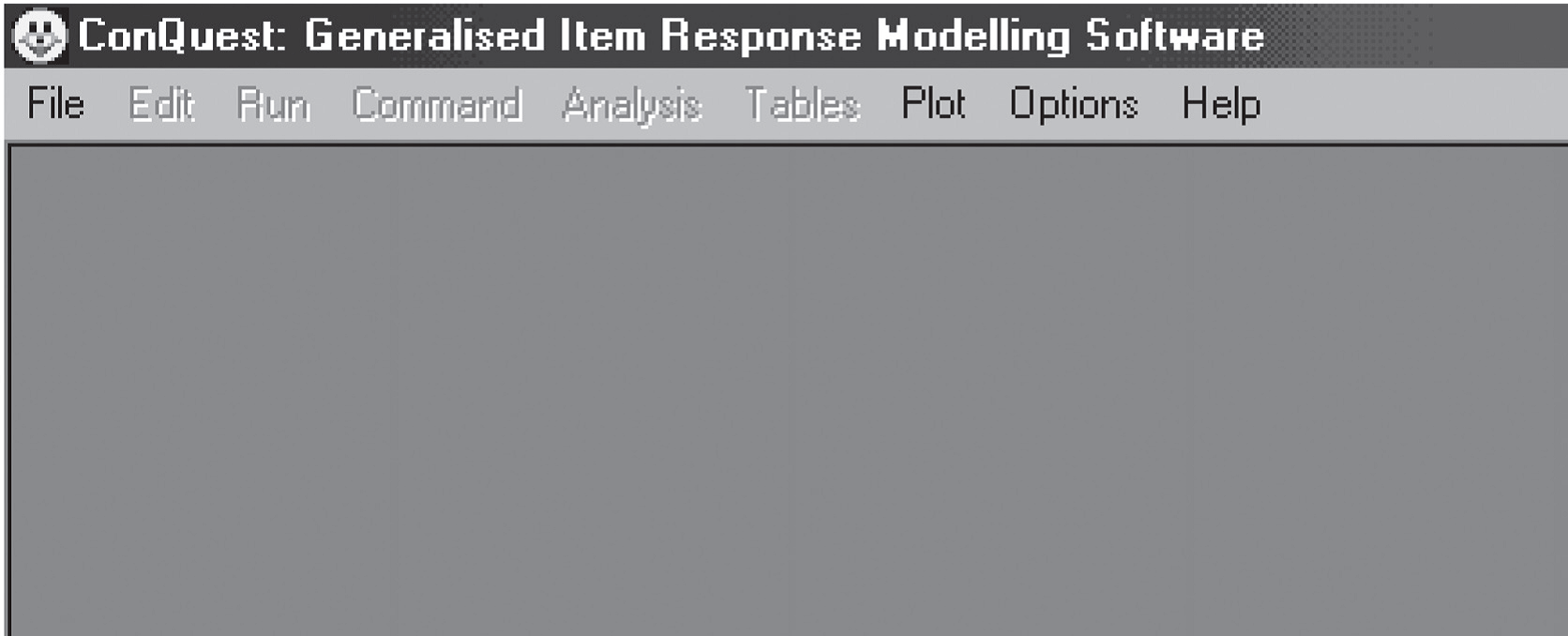
Figure 2.1: The ACER ConQuest Screen at Startup

If you choose to open an existing command file, a standard Windows File/Open dialog box will appear (see Figure 2.2). Locate the file you want to open. Note that, by default, the list of files will be restricted to those with the extension .cqc, which is the default extension for ACER ConQuest command files. To list other files, change the file type to All Files.

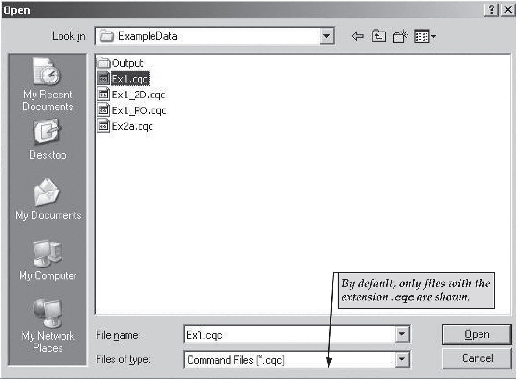
Figure 2.2: File/Open Dialog Box

If you choose to read a previously created system file, a standard Windows File/Open dialog box will appear. Locate the file you want to open. Note that, by default, the list of files will be restricted to those with the extension .CQS, which is the default extension for ACER ConQuest system files.

If you choose to create a new command file, or after you have selected an existing command file or system file from the File/Open dialog box, two windows will be created: an input window and an output window. These windows are illustrated in Figure 2.3.

A status bar reporting on the current activity of the program is located at the bottom of the ACER ConQuest window.

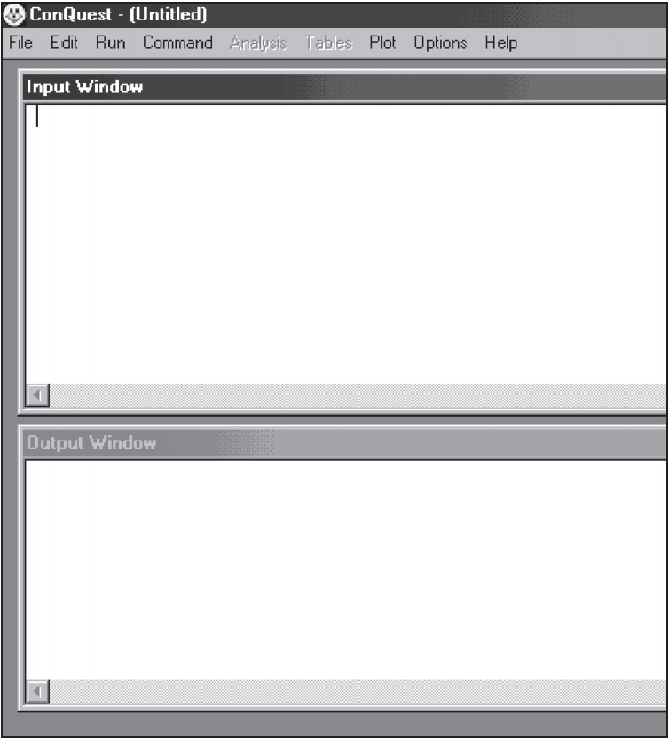
Figure 2.3: The ACER ConQuest Input and Output Windows

2.1.1.1 The Input Window

The input window is an editing window. If you have opened an existing ACER ConQuest command file, it will contain the file. If you have opened a system file or selected new, the input window will be blank.

Type or edit the ACER ConQuest command statements in the input window. To start execution of the command statements, choose Run\(\rightarrow\)Run All, if you wish to run all of the commands in the input window. To execute a subset of the commands then highlight the desired commands, choose Run\(\rightarrow\)Run Selection. ACER ConQuest will execute the command statements that are selected. This is illustrated in Figure 2.4. If nothing is highlighted, then ACER ConQuest will not execute any commands.

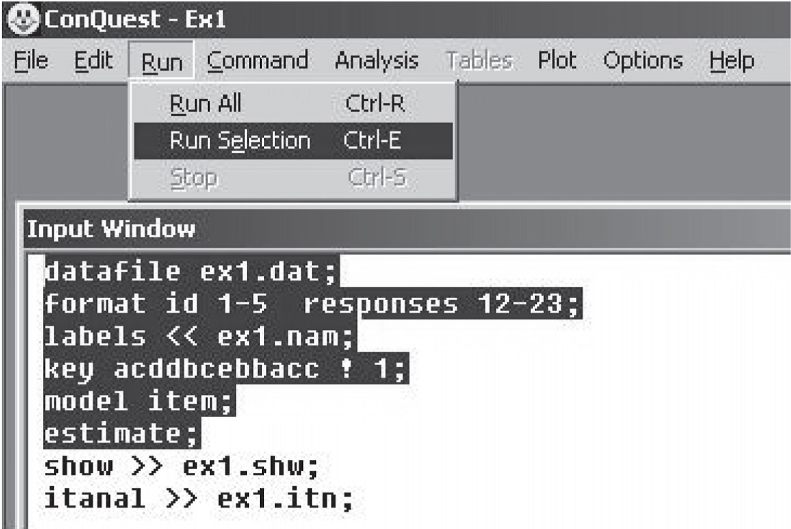
Figure 2.4: Running a Selection

2.1.1.2 The Output Window

The output window displays the results and the progress of the execution of the command statements. As statements are executed by ACER ConQuest, they are echoed in the output window. When ACER ConQuest is estimating item response models, progress information is displayed in the output window. Certain ACER ConQuest statements produce displays of the results of analyses. Unless these results are redirected to a file, they will be shown in the output window.

The output window has a limited amount of buffer space. When the buffer is full, material from the top of the buffer will be deleted. The contents of the buffer can be saved or edited at any time that ACER ConQuest is not busy undertaking computations. The output is cleared whenever Run\(\rightarrow\)Run All is chosen to execute all statements in the input window, whenever ACER ConQuest executes a reset statement, and whenever Command\(\rightarrow\)Clear Output is selected.

2.1.1.3 Using the Menus and Commands

The menus listed in the menu bar have several characteristics familiar to Windows users. The menus are drop-down menus. Menus are closed by either selecting a command or pressing the Esc key. Menus can be activated by pressing the Alt key plus the underlined character in the menu name. A command can then be selected by pressing the underlined character in the command name. Keyboard shortcuts are indicated next to the commands.

Only one file can be open at any time.

2.1.1.4 Description of the Input Window Menu Items

When the input window is the active window, the menu bar contains the following items:

File, Edit, Run, Command, Analysis, Tables, Plot, Options, and Help
The majority of the items under these menus, which are for controlling ACER ConQuest’s data specification, estimation and result display, are described in detail in other sections. Note that this section describes the commands that are not described elsewhere in the manual.
File\(\rightarrow\)New
Creates a new input and output window. If you already have a file displayed in the input window, you will be prompted to save any changes, if necessary, before ACER ConQuest closes that file and creates a new input and output window.
File\(\rightarrow\)Open
Opens an existing ACER ConQuest command file and places it in the input window. If you already have a file displayed in the input window, you will be prompted to save any changes, if necessary, before ACER ConQuest closes that file and displays the File/Open dialog box.
File\(\rightarrow\)Save
Saves the contents of the input window under the current file name or prompts for a new file name if you have not yet named the file.
File\(\rightarrow\)Save As
Prompts for a new file name and saves the contents of the input window under the new file name.
File\(\rightarrow\)Print
Sends the contents of the input window to the printer.
File\(\rightarrow\)Exit
Terminates the ACER ConQuest program. If you have a file displayed in the input window, you will be prompted to save any changes, if necessary, before ACER ConQuest terminates.
Edit\(\rightarrow\)Undo, Edit\(\rightarrow\)Cut, Edit\(\rightarrow\)Copy, Edit\(\rightarrow\)Paste, Edit\(\rightarrow\)Delete, Edit\(\rightarrow\)Select All, Edit\(\rightarrow\)Font
These are standard Windows editing commands. The Edit\(\rightarrow\)Undo command undoes the most recent edit only.
Run\(\rightarrow\)Run All
Starts execution of all of the command statements that are contained in the input window.
Run\(\rightarrow\)Run Selection
Starts execution of the command statements that are completely highlighted. If nothing is highlighted, ACER ConQuest will execute all the command statements in the input window. Note that complete and legal commands, or sets of commands, must be highlighted, if only part of a statement is highlighted, ACER ConQuest will display an error message.
Run\(\rightarrow\)Stop
Interrupts a current analysis
Plot\(\rightarrow\)Launch PlotQuest
Starts the ACER ConQuest plotting program
Options\(\rightarrow\)Display Progress
Toggles display of a dialog box that reports on estimation progress.
Help\(\rightarrow\)About this program
Shows the version number of the ACER ConQuest program you are using.

2.1.1.5 Description of the Output Window Menu Items

When the output window is the active window, the menu bar displays the following commands:

File\(\rightarrow\)Save
Saves the contents of the output window under the current file name or prompts for a new file name if you have not yet named the file.
File\(\rightarrow\)Save As
Prompts for a new file name and saves the contents of the output window under the new file name.
File\(\rightarrow\)Print
Sends the contents of the output window to the printer.

2.1.2 Console Version

The console version of ACER ConQuest provides a command line interface that does not draw upon the GUI features of the host operating system. This version of ACER ConQuest is substantially faster than the GUI version but is more limited in its functionality.

Figure 2.5 shows the screen when the console version of ACER ConQuest is started (double-click on the file ConQuestConsole.exe). The less than character (<) is the ACER ConQuest prompt. When the ACER ConQuest prompt is displayed, any appropriate ACER ConQuest statement can be entered. As with any command line interface, ACER ConQuest attempts to execute the command statement when you press the Enter key. If you have not yet entered a semi-colon (;) to indicate the end of the statement, the ACER ConQuest prompt changes to a plus sign (+) to indicate that the statement is continuing on a new line.

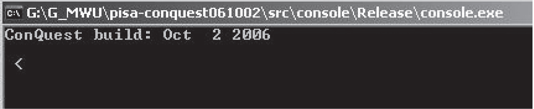
Figure 2.5: The Console ACER ConQuest Screen at Startup

The syntax of ACER ConQuest commands is described in section 4.1, and the remaining sections in this section illustrate various sets of command statements.

To exit from the ACER ConQuest program, enter the statement quit; at the ACER ConQuest prompt.

On many occasions, a file containing a set of ACER ConQuest statements (an ACER ConQuest command file) will be prepared with a text editor, and you will want ACER ConQuest to run the set of statements that are in the file. For example if the file is called myfile.cqc, then the statements in the file can be executed in two ways.

In the first method, start ACER ConQuest (see the Installation Instructions if you don’t know how to start ACER ConQuest) and then type the command
```
submit myfile.cqc;
```
A second method, which will work on operating systems that allow ACER ConQuest to be launched from a command line interface, is to provide the command file as a command line argument. That is, launch ACER ConQuest using
```
ConQuestCMD myfile.cqc;
```

With either method, after you press the Enter key, ACER ConQuest will proceed to execute each statement in the file. As statements are executed, they will be echoed on the screen. If you have requested displays of the analysis results and have not redirected them to a file, they will be displayed on the screen.

ACER ConQuest system files can be exchanged between the console and GUI versions. For large analyses it may be advantageous to fit the model with the console version, save a system file and then read that system file with the GUI version, for the purpose of preparing output plots and other displays.

2.1.3 Temporary Files

While ACER ConQuest is running, a number of temporary files will be created. These files have prefix “laji” (e.g., laji000.1, laji002.1, etc.). ACER ConQuest removes these files before closing the program. If these temporary files remain when ACER ConQuest is not running, you should remove them, as these files are typically large in size.

2.2 A Dichotomously Scored Multiple Choice Test

Multiple choice items are perhaps the most widely applied tool in testing. This is particularly true in the case of the testing of the cognitive abilities or achievements of a group of students.³ The analysis of the basic properties of dichotomous items and of tests containing a set of dichotomous items is the simplest application of ACER ConQuest. This first sample analysis, shows how ACER ConQuest can be used to fit Rasch’s simple logistic model to data gathered with a multiple choice test. ACER ConQuest can also generate a range of traditional test item statistics.⁴

2.2.1 Required files

The files used in this sample analysis are:

filename	content
ex1.cqc	The command statements.
ex1_dat.txt	The data.
ex1_lab.txt	The variable labels for the items on the multiple choice test.
ex1_shw.txt	The results of the Rasch analysis.
ex1_itn.txt	The results of the traditional item analyses.

(The last two files are created when the command file is executed.)

The data used in this tutorial comes from a 12-item multiple-choice test that was administered to 1000 students. The data have been entered into the file ex1_dat.txt, using one line per student. A unique student identification code has been entered in columns 1 through 5, and the students’ responses to each of the items have been recorded in columns 12 through 23. The response to each item has been allocated one column; and the codes a, b, c and d have been used to indicate which alternative the student chose for each item. If a student failed to respond to an item, an M has been entered into the data file. An extract from the data file is shown in Figure 2.6.

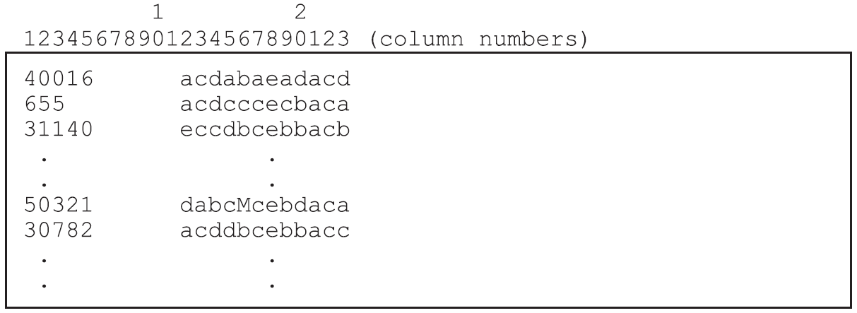
Extract from the Data File ex1_dat.txt. Each column of the data file is labelled so that it can be easily referred to in the text. The actual ACER ConQuest data file does not have any column labels.

Figure 2.6: Extract from the Data File ex1_dat.txt. Each column of the data file is labelled so that it can be easily referred to in the text. The actual ACER ConQuest data file does not have any column labels.

2.2.2 Syntax

In this sample analysis, the Rasch (1980) simple logistic model will be fitted to the data, and traditional item analysis statistics are generated. ex1.cqc is the command file used in this tutorial, and is shown in the code box below. A list explaining each line of syntax follows.

The syntax for ACER ConQuest commands is presented in section 4.1.

ex1.cqc:

datafile ex1_dat.txt;
format id 1-5 responses 12-23;
labels << ex1_lab.txt;
key acddbcebbacc ! 1;
model item;
estimate;
show >> results/ex1_shw.txt;
itanal >> results/ex1_itn.txt;
/* rout option is for use in R using conquestr: */
plot icc ! rout=results/icc/ex1_;
plot mcc! legend=yes;

Line 1
The datafile statement indicates the name and location of the data file. Any file name that is valid for the operating system you are using can be used here.
Line 2
The format statement describes the layout of the data in the file ex1_dat.txt. This format statement indicates that a field that will be called id is located in columns 1 through 5 and that the responses to the items are in columns 12 through 23 of the data file. Every format statement must give the location of the responses. In fact, the explicit variable responses must appear in the format statement or ACER ConQuest will not run. In this particular sample analysis, the responses are those made by the students to the multiple choice items; and, by default, item will be the implicit variable name that is used to indicate these responses. The levels of the item variable (that is, item 1, item 2 and so on) are implicitly identified through their location within the set of responses (called the response block) in the format statement; thus, in this sample analysis, the data for item 1 is located in column 12, the data for item 2 is in column 13, and so on.

EXTENSION: The item numbers are determined by the order in which the column locations are set out in the response block. If you use the following:
format id 1-5 responses 12-23;
item 1 will be read from column 12. If you use:
format id 1-5 responses 23,12-22;
item 1 will be read from column 23

TIP: In some testing contexts, it may be more informative to refer to the response variable as something other than item. Using the variable name task or question may lead to output that is better documented. Altering the name of the response variable is easy. If you want to use the name tasks rather than item, simply add an option to the format statement as follows:
format id 1-5 responses 12-23 ! tasks(12);
The variable name tasks must then be used to indicate the response variable in other ACER ConQuest commands. For example in the model statement in Line 5.
Line 3
The labels statement indicates that a set of labels for the variables (in this case, the items) is to be read from the file ex1_lab.txt. An extract of ex1_lab.txt is shown in Figure 2.7. (This file must be text only; if you create or edit the file with a word processor, make sure that you save it using the text only option.) The first line of the file contains the special symbol ===> (a string of three equals signs and a greater than sign) followed by one or more spaces and then the name of the variable to which the labels are to apply (in this case, item). The subsequent lines contain two pieces of information separated by one or more spaces. The first value on each line is the level of the variable (in this case, item) to which a label is to be attached, and the second value is the label. If a label includes spaces, then it must be enclosed in double quotation marks (“ “). In this sample analysis, the label for item 1 is BSMMA01, the label for item 2 is BSMMA02, and so on.

TIP: Labels are not required by ACER ConQuest, but they improve the readability of any ACER ConQuest printout, so their use is strongly recommended.

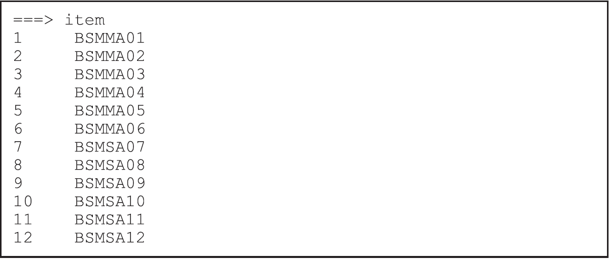
Figure 2.7: Contents of the Label File ex1_lab.txt.

Line 4
The key statement identifies the correct response for each of the multiple choice test items. In this case, the correct answer for item 1 is a, the correct answer for item 2 is c, the correct answer for item 3 is d, and so on. The length of the argument in the key statement is 12 characters, which is the length of the response block given in the format statement.

If a key statement is provided, ACER ConQuest will recode the data so that any response a to item 1 will be recoded to the value given in the key statement option (in this case, 1). All other responses to item 1 will be recoded to the value of the key_default (in this case, 0). Similarly, any response c to item 2 will be recoded to 1, while all other responses to item 2 will be recoded to 0; and so on.
Line 5
The model statement must be provided before any traditional or item response analyses can be undertaken. When undertaking simple analyses of multiplechoice tests, as in this example, the argument for the model statement is the name of the variable that identifies the response data that are to be analysed (in this case, item).
Line 6
The estimate statement initiates the estimation of the item response model.

NOTE: The order in which commands can be entered into ACER ConQuest is not fixed. There are, however, logical constraints on the ordering. For example, show statements cannot precede the estimate statement, which in turn cannot precede the model, format or datafile statements.
Line 7
The show statement produces a sequence of tables that summarise the results of fitting the item response model. In this case, the redirection symbol (>>) is used so that the results will be written to the file ex1_shw.txt in your current directory. If redirection is omitted, the results will be displayed on the console (or in the output window for the GUI version).
Line 8
The itanal statement produces a display of the results of a traditional item analysis. As with the show statement, the results are redirected to a file (in this case, ex1_itn.txt).
Line 10
The Plot icc statement will produce 12 item characteristic curve plots, one for each item. The plots will compare the modelled item characteristic curves with the empirical item characteristic curves. Note that this command is not available in the console version of ACER ConQuest.
Line 11
The Plot mcc statement will produce 12 category characteristic curve plots, one for each item. The plots will compare the modelled item characteristic curves with the empirical item characteristic curves (for correct answers) and will also show the behavior of the distractors. Note that this command is not available in the console version of ACER ConQuest.

2.2.3 Running the Multiple Choice Sample Analysis

To run this sample analysis, start the GUI version. Open the file ex1.cqc and choose Run\(\rightarrow\)Run All.

Alternatively, you can launch the console version of ACER ConQuest, by typing the command⁵ (on Windows) ConQuestConsole.exe ex1.cqc.

ACER ConQuest will begin executing the statements that are in the file ex1.cqc and as they are executed, they will be echoed on the screen (or output window). When ACER ConQuest reaches the estimate statement, it will begin fitting Rasch’s simple logistic model to the data, and as it does so it will report on the progress of the estimation. Figure 2.8 is an extract of the information that is provided during the estimation (in this case, the changes in the estimates after four iterations).

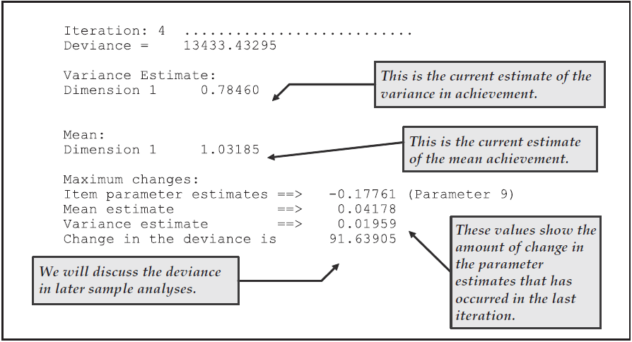
Figure 2.8: Reported Information on the Progress of Estimation

After the estimation is completed, the two statements that produce text output (show and itanal) will be processed and then, in the case of the GUI version two sets of 12 plots will be produced. In this case, the show statement will produce all six of its tables. All of these tables will be in the file ex1_shw.txt. The contents of the first table are shown in Figure 2.9.

This table is provided for cross-referencing and record-keeping purposes. It indicates the data set that was analysed, the format that was used to read the data, the model that was requested and the sample size. It also provides the number of parameters that were estimated, the number of iterations that the estimation took, and the reason for the termination of the estimation. The deviance is a statistic that indicates how well the item response model has fit the data; it will be discussed further in future sample analyses.

As Figure 2.9 shows, in this analysis 13 parameters were estimated. They are: (a) the mean and variance of the latent achievement that is being measured by these items; and (b) 11 item difficulty parameters. Following the usual convention of Rasch modelling, the mean of the item difficulty parameters has been made zero, so that a total of 11 parameters is required to describe the difficulties of the 12 items.

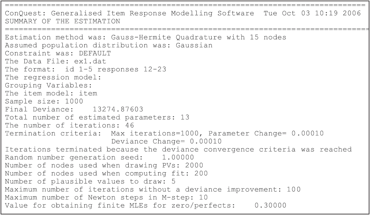
Figure 2.9: Summary Table

Figure 2.10 shows the second table from the file ex1_shw.txt. This table gives the parameter estimates for each of the test items along with their standard errors and some diagnostics tests of fit. The estimation algorithm and the methods used for computing standard errors and fit statistics are discussed in Chapter 3. In brief, the item parameter estimates are marginal maximum likelihood estimates obtained using an EM algorithm, the standard errors are asymptotic estimates given by the inverse of the hessian, and the fit statistics are residual-based indices that are similar in conception and purpose to the weighted and unweighted fit statistics that were developed by Wright & Stone (1979) and Wright & Masters (1982) for Rasch’s simple logistic model and the partial credit model respectively.

For the MNSQ fit statistics we provide a ninety-five percent confidence interval for the expected value of the MNSQ (which under the null hypothesis is 1.0). If the MNSQ fit statistic lies outside that interval then we reject the null hypothesis that the data conforms to the model. If the MNSQ fit statistic lies outside the interval then the corresponding T statistics will have an absolute value that exceeds 2.0.

At the bottom of the table an item separation reliability and chi-squared test of parameter equality are reported. The separation reliability is as described in Wright & Stone (1979). This indicates how well the item parameters are separated; it has a maximum of one and a minimum of zero. This value is typically high and increases with increasing sample sizes. The null hypothesis for the chi-square test is equality of the set of parameters. In this case equality of all of the parameters is rejected because the chi-square is significant. This test is not useful here, but will be of use in other contexts, where parameter equivalence (e.g., rater severity) is of concern.

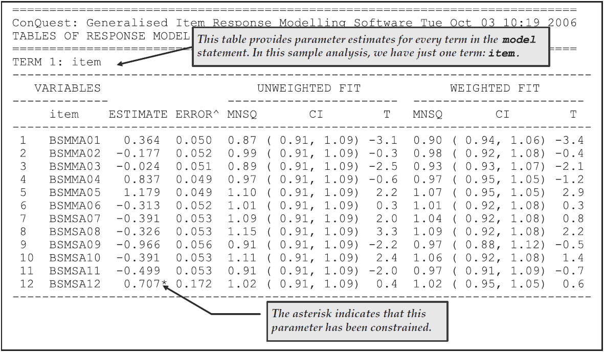
Figure 2.10: The Item Parameter Estimates

The third table in the show statement’s output (not shown for the sake of brevity) gives the estimates of the population parameters. In this case, these are simply estimates of the mean of the latent ability distribution and of the variance of that distribution. In this case, the mean is estimated as 1.070, and the variance is estimated as 0.866.

Extension: In Rasch modelling, it is usual to identify the model by setting the mean of the item difficulty parameters to zero. This is also the default behaviour for ACER ConQuest, which automatically sets the value of the ‘last’ item parameter to ensure an average of zero. In ACER ConQuest, however, you can, as an alternative, choose to set the mean of the latent ability distribution to zero. To do this, use the set command as follows:
set lconstraints=cases;
If you want to use a different item as the constraining item, then you can read the items in a different order. For example:
format id 1-5 responses 12-15, 17-23, 16;
would result in the constraint being applied to the item in column 16. But be aware, it will now be called item 12, not item 5, as it is the twelfth item in the response block.

This table also provides a set of reliability indices.

The fourth table in the output, Figure 2.11, provides a map of the item difficulty parameters.

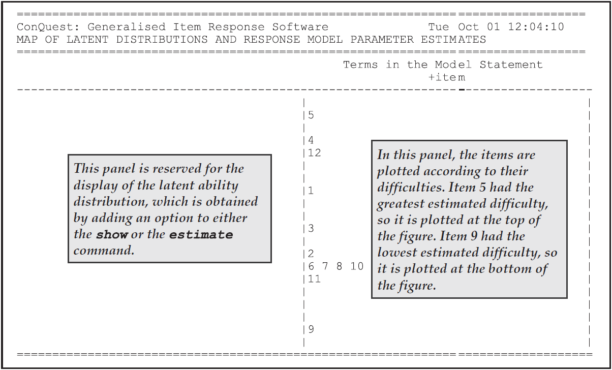
Figure 2.11: The Item and Latent Distribution Map for the Simple Logistic Model

The file ex1_shw.txt contains one additional table, labelled Map of Latent Distributions and Thresholds. In the case of dichotomously scored items and a model statement with a single term⁶, these maps provide the same information as that shown in Figure 2.11, so they are not discussed further.

The traditional item analysis is invoked by the itanal statement, and its results have been written to the file ex1_itn.txt. The itanal output includes a table showing classical difficulty, discrimination, and point-biserial statistics for each item. Figure 2.12 shows the results for item 2.

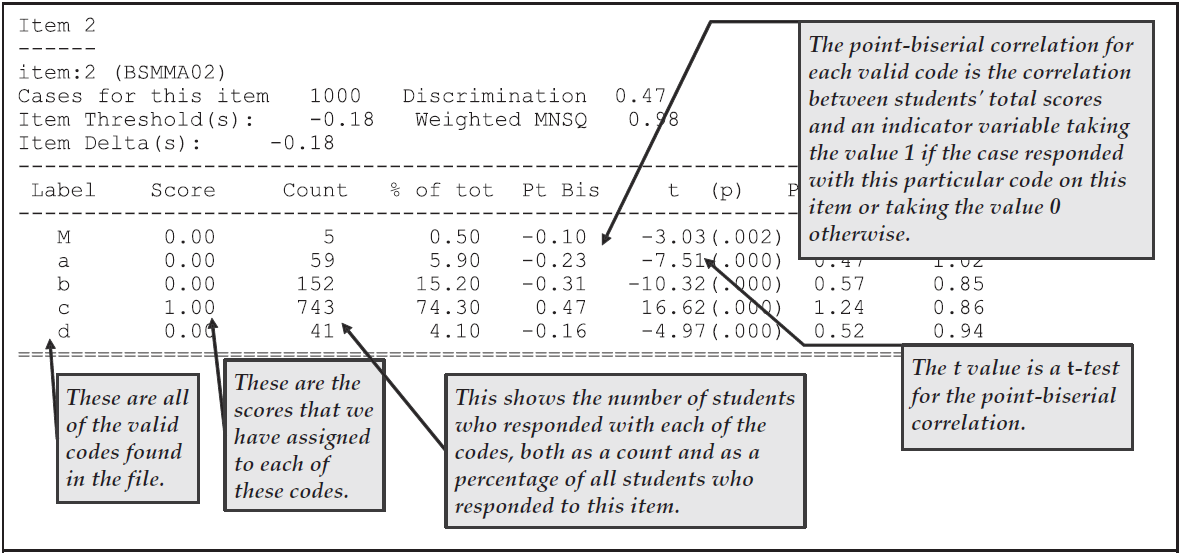
Figure 2.12: Example of Traditional Item Analysis Results

Summary results, including coefficient alpha for the test as a whole, are printed at the end of the file ex1_itn.txt as shown in Figure 2.13. Discussion of the usage of the statistics can be found in any standard text book, such as Crocker & Algina (1986).

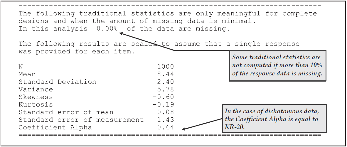
Figure 2.13: Summary Statistics from Traditional Item Analysis Results

Figure 2.14 shows one of the 12 plots that were produced by the plot icc command. The ICC plot shows a comparison of the empirical item characteristic curve (the broken line, which is based directly upon the observed data) with the modelled item characteristic curve (the smooth line).

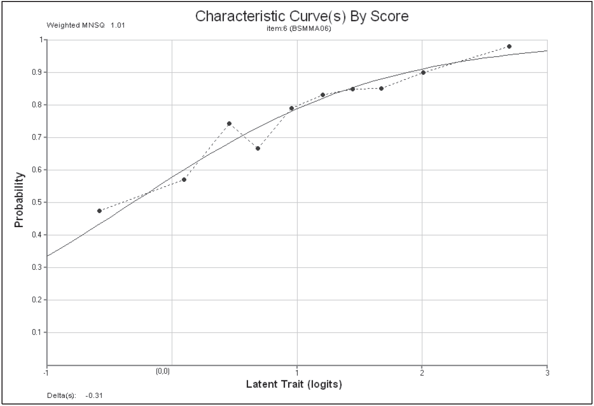
Figure 2.14: Modelled and Empirical Item Characteristic Curves for Item 6

Figure 2.15 shows a matching plot produced by the plot mcc command. In addition to showing the modelled curve and the matching empirical curve, this plot shows the characteristics of the incorrect responses—the distractors. In particular it shows the proportion of students in each of a sequence of ten ability groupings⁷ that responded with each of the possible responses.

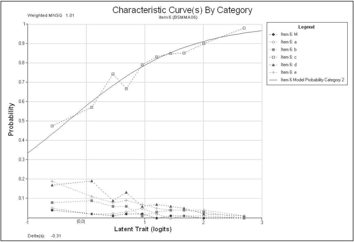
Figure 2.15: Modelled and Empirical Category Characteristics Curves for Item 6

TIP: Whenever a key statement is used, the itanal statement will display results for all valid data codes. If a key statement is not used, the itanal statement will display the results of an analysis done after recoding has been applied.

2.2.4 Summary

This section shows how ACER ConQuest can be used to analyse a multiple-choice test. Some key points covered in this section are:

the datafile, format and model statements are prerequisites for data set analysis.
the key statement provides an efficient method for scoring multiple choice tests.
the estimate statement is used to fit an item response model to the data.
the itanal statement generates traditional item statistics.
the plot statement displays graphs which illustrate the relationship between the empirical data and the model’s expectation.

EXTENSION: ACER ConQuest can fit other models to multiple choice tests, including models such as the ordered partition model.

2.3 Modelling Polytomously Scored Items with the Rating Scale and Partial Credit Models

The rating scale model (Andrich, 1978; Wright & Masters, 1982) and the partial credit model (Masters, 1982; Wright & Masters, 1982) are extensions to Rasch’s simple logistic model and are suitable for use when items are scored polytomously. The rating scale model was initially developed by Andrich for use with Likert-style items, while Masters’ extension of the rating scale model to the partial credit model was undertaken to facilitate the analysis of cognitive items that are scored into more than two ordered categories. In this section, the use of ACER ConQuest to fit the partial credit and rating scale models is illustrated through two sets of sample analyses. In the first, the partial credit model is fit to some cognitive items; and in the second, the fit of the rating scale and partial credit models to a set of items that forms an attitudinal scale is compared.

2.3.1 a) Fitting the Partial Credit Model

The data for the first sample analysis are the responses of 515 students to a test of science concepts related to the Earth and space. Previous analyses of some of these data are reported in Adams et al. (1991).

2.3.1.1 Required files

The files used in this sample analysis are:

filename	content
ex2a.cqc	The command statements.
ex2a_dat.txt	The data.
ex2a_lab.txt	The variable labels for the items on the partial credit test.
ex2a_shw.txt	The results of the partial credit analysis.
ex2a_itn.txt	The results of the traditional item analyses.

(The last two files are created when the command file is executed.)

The data have been entered into the file ex2a_dat.txt, using one line per student. A unique identification code has been entered in columns 2 through 7, and the students’ response to each of the items has been recorded in columns 10 through 17. In this data, the upper-case alphabetic characters A, B, C, D, E, F, W, and X have been used to indicate the different kinds of responses that students gave to these items. The code Z has been used to indicate data that cannot be analysed. For each item, these codes are scored (or, more correctly, mapped onto performance levels) to indicate the level of quality of the response. For example, in the case of the first item (the item in column 10), the response coded A is regarded as the best kind of response and is assigned to level 2, responses B and C are assigned to level 1, and responses W and X are assigned to level 0. An extract of the file ex2a_dat.txt is shown in Figure 2.16.

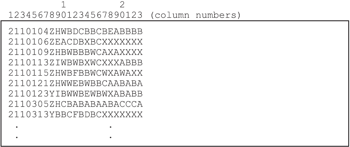
Figure 2.16: Extract from the Data File ex2a_dat.txt

NOTE: In most Rasch-type models, a one-to-one match exists between the label that is assigned to each response category to an item (the category label) and the response level (or score) that is assigned to that response category. This need not be the case with ACER ConQuest.

In ACER ConQuest, the distinction between a response category and a response level is an important one. When ACER ConQuest fits item response models, it actually models the probabilities of each of the response categories for each item. The scores for each of these categories need not be unique. For example, a four-alternative multiple choice item can be modelled as a four-response category item with three categories assigned zero scores and one category assigned a score of one, or it can be modelled in the usual fashion as a two-category item where the scores identify the categories.

2.3.1.2 Syntax

The command file used in this analysis of a Partial Credit Test is ex2a.cqc, which is shown in the code box below. Each line of the command file is described in the list underneath the code box.

ex2a.cqc:

Title Partial Credit Model: What happened last night;
data ex2a_dat.txt;
format name 2-7 responses 10-17;
labels << ex2a_lab.txt;
codes 3,2,1,0;
recode (A,B,C,W,X) (2,1,1,0,0)            !items(1);
recode (A,B,C,W,X) (3,2,1,0,0)            !items(2);
recode (A,B,C,D,E,F,W,X) (3,2,2,1,1,0,0,0)!items(3);
recode (A,B,C,W,X) (2,1,0,0,0)            !items(4);
recode (A,B,C,D,E,W,X) (3,2,1,1,1,0,0)    !items(5);
recode (A,B,W,X) (2,1,0,0)                !items(6);
recode (A,B,C,W,X) (3,2,1,0,0)            !items(7);
recode (A,B,C,D,W,X) (3,2,1,1,0,0)        !items(8);
model item + item*step;
estimate;
show !estimates=latent >> results/ex2a_shw.txt;
itanal >> results/ex2a_itn.txt;
plot expected! gins=2;
plot icc! gins=2;
plot ccc! gins=2;

Line 1
Gives a title for this analysis. The text supplied after the command title will appear on the top of any printed ACER ConQuest output. If a title is not provided, the default, ConQuest: Generalised Item Response Modelling Software, will be used.
Line 2
Indicates the name and location of the data file. Any name that is valid for the operating system you are using can be used here.
Line 3
The format statement describes the layout of the data in the file ex2a_dat.txt. This format indicates that a field called name is located in columns 2 through 7 and that the responses to the items are in columns 10 through 17 (the response block) of the data file.
Line 4
A set of labels for the items are to be read from the file ex2a_lab.txt. If you take a look at these labels, you will notice that they are quite long. ACER ConQuest labels can be of any length, but most ACER ConQuest printouts are limited to displaying many fewer characters than this. For example, the tables of parameter estimates produced by the show statement will display only the first 11 characters of the labels.
Line 5
The codes statement is used to restrict the list of codes that ACER ConQuest will consider valid. In the sample analysis in section 2.2, a codes statement was not used. This meant that any character in the response block defined by the format statement — except a blank or a period (.) character (the default missing-response codes) — was considered valid data. In this sample analysis, the valid codes have been limited to the digits 0, 1, 2 and 3; any other codes for the items will be treated as missing-response data. It is important to note that the codes statement refers to the codes after the application of any recodes.
Lines 6-13
The eight recode statements are used to collapse the alphabetic response categories into a smaller set of categories that are labelled with the digits 0, 1, 2 and 3. Each of these recode statements consists of three components:
- The first component is a list of codes contained within parentheses. These are codes that will be found in the data file ex2a_dat.txt, and these are called the from codes.
- The second component is also a list of codes contained within parentheses, these codes are called the to codes. The length of the to codes list must match the length of the from codes list. When ACER ConQuest finds a response that matches a from code, it will change (or recode) it to the corresponding to code.
- The third component (the option of the recode command) gives the levels of the variables for which the recode is to be applied. Line 11, for example, says that, for item 6, A is to be recoded to 2, B is to be recoded to 1, and W and X are both to be recoded to 0.
Any codes in the response block of the data file that do not match a code in the from list will be left untouched. In these data, the Z codes are left untouched; and since Z is not listed as a valid code, all such data will be treated as missing-response data.

When ACER ConQuest models these data, the number of response categories that will be assumed for each item will be determined from the number of distinct codes for that item. Item 1 has three distinct codes (2, 1 and 0), so three categories will be modelled; item 2 has four distinct codes (3, 2, 1 and 0), so four categories will be modelled.
Line 14
The model statement for these data contains two terms (item and item*step) and will result in the estimation of two sets of parameters. The term item results in the estimation of a set of item difficulty parameters, and the term item*step results in a set of item step-parameters that are allowed to vary across the items. This is the partial credit model.

In the section [The Structure of ACER ConQuest Design Matrices] in chapter 3, there is a description of how the terms in the model statement specify different versions of the item response model.
Line 15
The estimate statement is used to initiate the estimation of the item response model.
Line 16
The show statement produces a display of the item response model parameter estimates and saves them to the file ex2a_shw.txt. The option estimates=latent requests that the displays include an illustration of the latent ability distribution.
Line 17
The itanal statement produces a display of the results of a traditional item analysis. As with the show statement, the results have been redirected to a file (in this case, ex2a_itn.txt).
Lines 18-20
The plot statements produce a sequence of three displays for item 2 only. The first requested plot is a comparison of the observed and the modelled expected score curve. The second plot is a comparison of the observed and modelled item characteristics curves, and the third plot shows comparisons of the observed and expected cumulative item characteristic curves.

2.3.1.3 Running the Partial Credit Sample Analysis

To run this sample analysis, start the GUI version. Open the file ex2a.cqc and choose Run\(\rightarrow\)Run All.

ACER ConQuest will begin executing the statements that are in the file ex2a.cqc; and as they are executed, they will be echoed on the screen. When ACER ConQuest reaches the estimate statement, it will begin fitting the partial credit model to the data, and as it does so it will report on the progress of the estimation.

After the estimation is complete, the two statements that produce output (show and itanal) will be processed. As in the previous sample analysis, the show statement will produce six separate tables. All of these tables will be in the file ex2a_shw.txt. The contents of the first table were discussed in section 2.2. The first half of the second table, which contains information related to the parameter estimates for the first term in the model statement, is shown in Figure 2.17. The parameter estimates in this table are for the difficulties of each of the items. For the purposes of model identification, ACER ConQuest constrains the difficulty estimate for the last item to ensure an average difficulty of zero. This constraint has been achieved by setting the difficulty of the last item to be the negative sum of the previous items. The fact that this item is constrained is indicated by the asterisk (*) placed next to the parameter estimate.

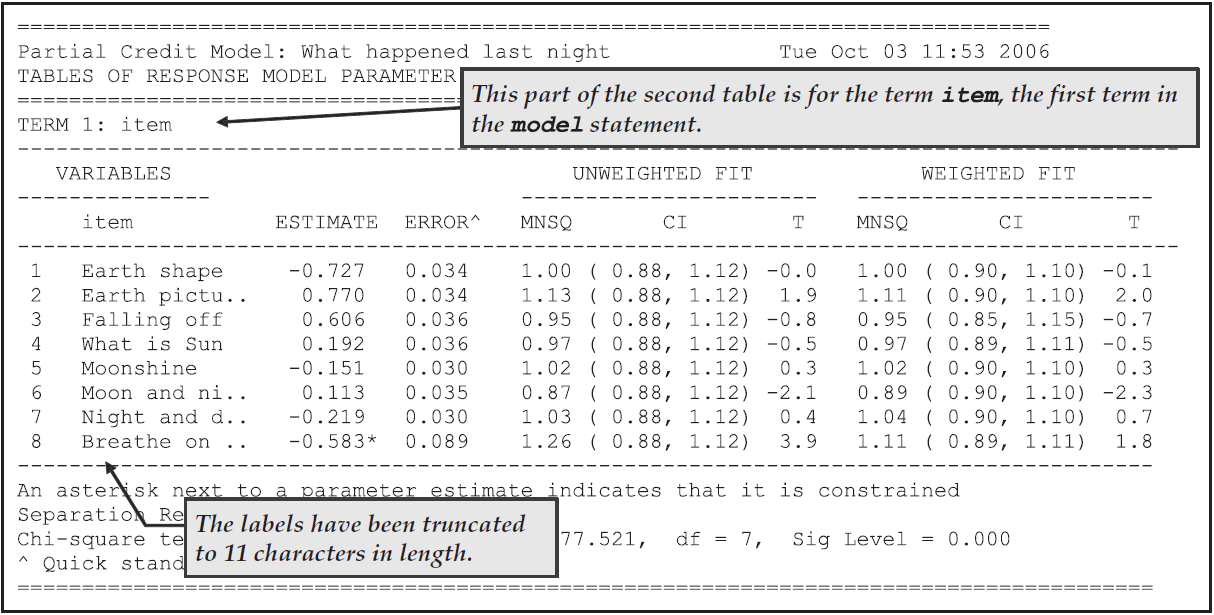
Figure 2.17: Parameter Estimates for the First Term in the model Statement

Figure 2.18 shows the second table, which displays the parameter estimates, standard errors and fit statistics associated with the second term in the model statement, the step parameters. You will notice that the number of step parameters that has been estimated for each item is one less than the number of modelled response categories for the item. Furthermore, the last of the parameters for each item is constrained so that the sum of the parameters for an item equals zero. This is a necessary identification constraint. In the case of item 1, for example, there are three categories, 0, 1 and 2. Two values are reported, but only the first step parameter has been estimated. The second is the negative of the first. The parameter labelled as step 1, describes the transition from category 0 to 1, where the probability of being in category 1 is greater than the probability of being in category 0, while the second step describes the transition from 1 to 2. The section The Structure of ACER ConQuest Design Matrices in Chapter 3 gives a description of why an item has two fewer step parameters than it has categories, and it discusses the interpretation of these parameters.

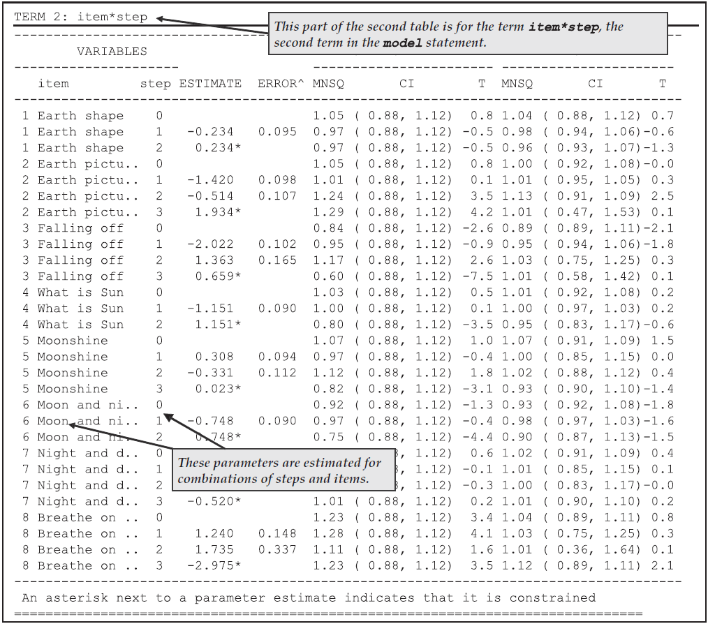
Figure 2.18: Parameter Estimates for the Second Term in the model Statement

There is a fit statistic reported for each category. This statistic provides a comparison of the expected number of students responding in the category with the observed number responding in that category.

The third table in the file (not shown here) gives the estimates of the population parameters. In this case, the mean of the latent ability distribution is –0.320, and the variance of that distribution is 0.526.

The fourth table reports the reliability coefficients. Three different reliability statistics are available (Adams, 2005). In this case just the third index (the EAP/PV reliability) is reported because neither of the maximum likelihood estimates has been computed at this stage. The reported reliability is 0.735.

The fifth table Figure 2.19 is a map of the parameter estimates and latent ability distribution. For this model, the map consists of two panels, one for the latent ability distribution and one for each of the terms in the model statement that do not include a step (in this case one). In this case the leftmost panel shows the estimated latent ability distribution and the second shows the item difficulties.

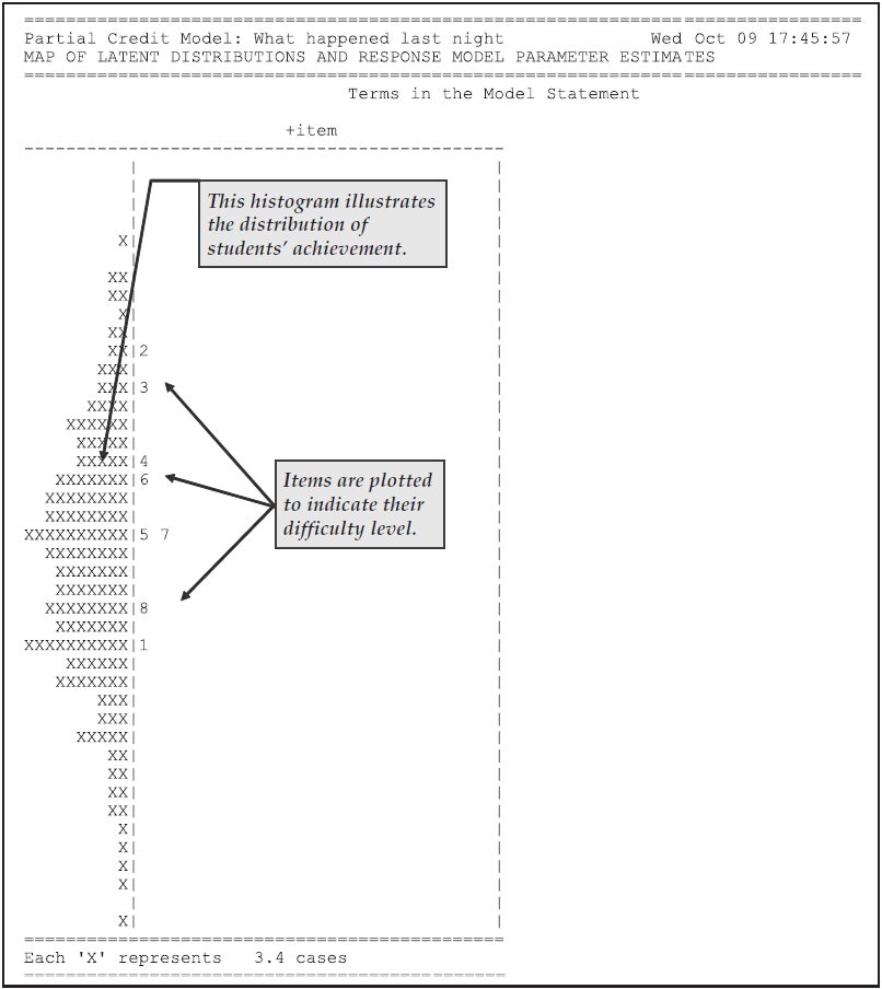
Figure 2.19: The Item and Latent Distribution Map for the Partial Credit Model

EXTENSION: The headings of the panels in Figure 2.19 are preceded by a plus sign (+). This indicates the orientation of the parameters. A plus indicates that the facet is modelled with difficulty parameters, whereas a minus sign (–) indicates that the facet is modelled with easiness parameters. This is controlled by the sign that you use in the model statement.

Figure 2.20, the sixth table from the file ex2a_shw.txt, is a plot of the Thurstonian thresholds for the items. The definition of these thresholds is discussed in Computing Thresholds in Chapter 3. Briefly, they are plotted at the point where a student has a 50% chance of achieving at least the indicated level of performance on an item.

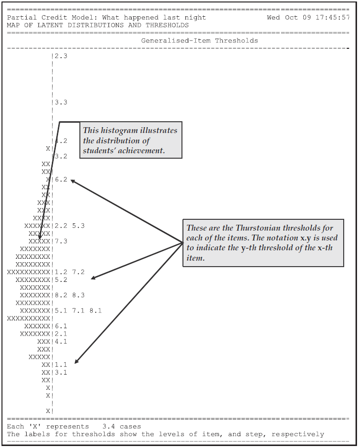
Figure 2.20: Item Thresholds for the Partial Credit Model

The itanal command in line 17 produces a file (ex2a_itn.txt) that contains traditional item statistics (Figure 2.21). In the previous section a multiple-choice test was analysed and the itanal output for multiple-choice items was described. In this example a key statement was not used and the items use partial credit scoring. As a consequence the itanal results are provided at the level of scores, rather than response categories.

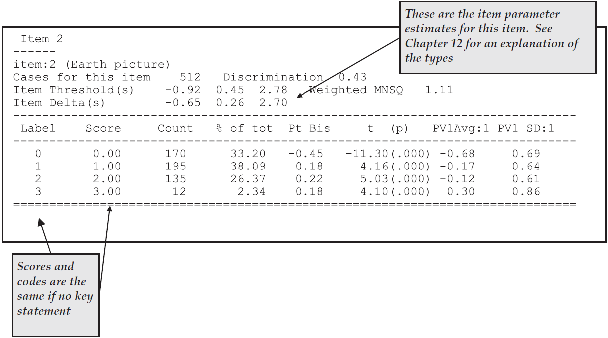
Figure 2.21: Extract of Item Analysis Printout for a Partial Credit Item

EXTENSION: The method used to construct the ability distribution is determined by the estimates= option used in the show statement. The latent distribution is constructed by drawing a set of plausible values for the students and constructing a histogram from the plausible values. Other options for the distribution are EAP, WLE and MLE, which result in histograms of expected a-posteriori, weighted maximum likelihood and maximum likelihood estimates, respectively. Details of these ability estimates are discussed in Latent Estimation and Prediction in Chapter 3.

The three plot commands (lines 18–20) produce the graphs shown in Figure 2.22. For illustrative purposes only plots for item 2 are requested. This item showed poor fit to the scaling model — in this case the partial credit model.

The item fit MNSQ of 1.11 indicates that this item is less discriminating than expected by the model. The first plot, the comparison of the observed and modelled expected score curves is the best illustration of this misfit. Notice how in this plot the observed curve is a little flatter than the modelled curve. This will often be the case when the MNSQ is significantly larger than 1.0.

The second plot shows the item characteristic curves, both modelled and empirical. There is one pair of curves for each possible score on the item, in this case 0, 1, 2 and 3. Note that the disparity between the observed and modelled curves for category 2 is the largest and this is consistent with the high fit statistic for this category.

The third plot is a cumulative form of the item characteristic curves. In this case three pairs of curves are plotted. The rightmost pair gives the probability of a response of 3, the next pair is for the probability of 2 or 3, and the final pairing is for the probability of 1, 2 or 3. Where these curves attain a probability of 0.5, the value on the horizontal axis corresponds to each of the three threshold parameters that are reported under the figure.

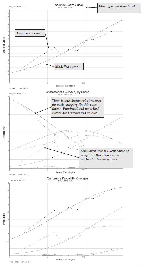
Figure 2.22: Plots for Item 2

2.3.2 b) Partial Credit and Rating Scale Models: A Comparison of Fit

A key feature of ACER ConQuest is its ability to fit alternative Rasch-type models to the same data set. Here a rating scale model and a partial credit model are fit to a set of items that were designed to measure the importance placed by teachers on adequate resourcing and support to the success of bilingual education programs.

2.3.2.1 Required files

The data come from a study undertaken by Zammit (1997). The data consist of the responses of 582 teachers to the 10 items listed in Figure 2.23. Each item was presented with a Likert-style response format; and in the data file, strongly agree was coded as 1, agree as 2, uncertain as 3, disagree as 4, and strongly disagree as 5.

Figure 2.23: Items Used in the Comparison of the Rating Scale and the Partial Credit Models

The files that we use are:

filename	content
ex2b.cqc	The command statements.
ex2b_dat.txt	The data.
ex2b_lab.txt	The variable labels for the items on the rating scale.
ex2b_shw.txt	The results of the rating scale analysis.
ex2b_itn.txt	The results of the traditional item analyses.
ex2c_shw.txt	The results of the partical credit analysis.

(The last three files are created when the command file is executed.)

2.3.2.2 Syntax

The code box below contains the contents of ex2b.cqc. This is the command file used in this analysis to fit a Rating Scale and then a Partial Credit Model to the same data we used in part a) of this tutorial. The list underneath the code box explains each line from the command file.

ex2b.cqc:

title Rating Scale Analysis;
datafile ex2b_dat.txt;
format responses 9-15,17-19;
codes 0,1,2;
recode (1,2,3,4,5) (2,1,0,0,0);
labels << ex2b_lab.txt;
model item + step;              /*Rating Scale*/
estimate;
show>>results/ex2b_shw.txt;
itanal>>results/ex2b_itn.txt;
reset;
title Partial Credit Analysis;
datafile ex2b_dat.txt;
format responses 9-15,17-19;
codes 0,1,2;
recode (1,2,3,4,5) (2,1,0,0,0);
labels << ex2b_lab.txt;
model item + item*step;         /*Partial Credit*/
estimate;
show>>results/ex2c_shw.txt;

Line 1
For this analysis, we are using the title Rating Scale Analysis.
Line 2
The data for this sample analysis are to be read from the file ex2b_dat.txt.
Line 3
The format statement describes the layout of the data in the file ex2b_dat.txt. This format indicates that the responses to the first seven items are located in columns 9 through 15 and that the responses to the next three items are located in columns 17 through 19.
Line 4
The valid codes, after recode, are 0, 1 and 2.
Line 5
The original codes of 1, 2, 3, 4, and 5 are recoded to 2, 1, and 0. Because 3, 4, and 5 are all being recoded to 0, this means we are collapsing these categories (uncertain, disagree, and strongly disagree) for the purposes of this analysis.
Line 6
A set of labels for the items is to be read from the file ex2b_lab.txt.
Line 7
This is the model statement that corresponds to the rating scale model. The first term in the model statement indicates that an item difficulty parameter is modelled for each item, and the second indicates that step parameters are the same for all items.
Line 8
The estimate statement is used to initiate the estimation of the item response model.
Line 9
Item response model results are to be written to the file ex2b_shw.txt.
Line 10
Traditional statistics are to be written to the file ex2b_itn.txt.
Line 11
The reset statement can be used to separate jobs that are put into a single command file. The reset statement returns all values to their defaults. Even though many values are the same for these analyses, we advise resetting, as you may be unaware of some values that have been set by the previous statements.
Lines 12-20
These lines replicate lines 1 to 9. The only difference is in the model statement (compare lines 18 and 7). In the first analysis, the second term of the model statement is step, whereas in the second analysis the second term is item*step. In the latter case, the step structure is allowed to vary across items, whereas in the first case, the step structure is constrained to be the same across items.

2.3.2.3 Running the Comparison of the Rating Scale and Partial Credit Models

To run this sample analysis, launch the GUI version of ACER ConQuest and open the command file ex2b.cqc and choose Run\(\rightarrow\)Run All.

ACER ConQuest will begin executing the statements that are in the file ex2b.cqc; and as they are executed, they will be echoed on the screen. Firstly the rating scale model will be fit, followed by the partial credit model.

To compare the fit of the two models to these data, two tables produced by the show statements for each model are compared. First, the summary tables for each model are compared. These two tables are reproduced in Figure 2.24. From these tables we note that the rating scale model has used 12 parameters, and the partial credit model has used 21 parameters. For the rating scale model, the parameters are the mean and variance of the latent variable, nine item difficulty parameters, and a single step parameter. For the partial credit model, the parameters are the mean and variance of the latent variable, nine item difficulty parameters and 10 step parameters.

A formal statistical test of the relative fit of these models can be undertaken by comparing the deviance of the two models. Comparing the deviance in the summary tables, note that the rating scale model deviance is 67.58 greater than the deviance for the partial credit model. If this value is compared to a chi-squared distribution with 9 degrees of freedom, this value is significant and it can be concluded that the fit of the rating scale model is significantly worse than the fit of the partial credit model.

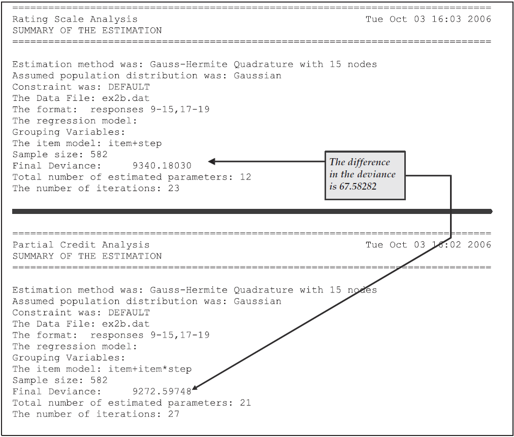
Figure 2.24: Summary Information for the Rating Scale and Partial Credit Analyses

The difference in the fit of these two models is highlighted by comparing the contents of Figures 2.25 and 2.26.

Figure 2.25 shows that, in the case of the rating scale model, the step parameter fits poorly, whereas in Figure 2.26 the fit statistics for the step parameters are generally small or less than their expected value (ie the t-values are negative). In both cases, the difficulty parameter for item 2 does not fit well. An examination of the text of this item in Figure 2.23 shows that perhaps the misfit of this item can be explained by the fact that it is slightly different to the other questions in that it focuses on the conditions under which a bilingual program should be started rather than on the conditions necessary for the success of a bilingual program. Thus, although overall the partial credit model fits better than the rating scale model as discussed previously, the persistence of misfit for the difficulty parameter for this item indicates that the inclusion of this item in the scale should be reconsidered.

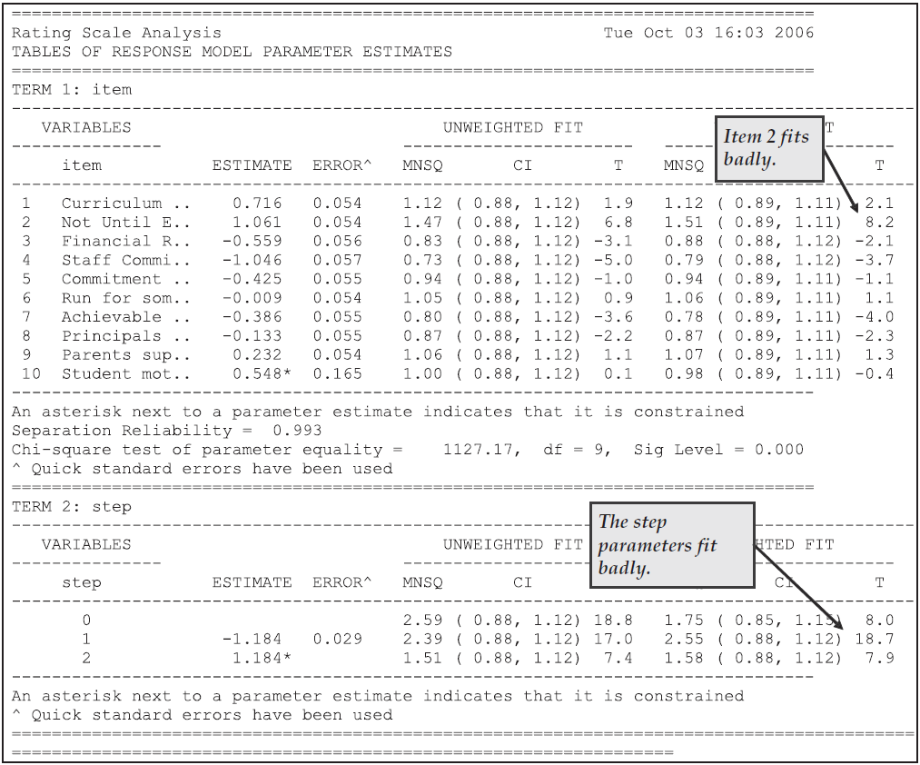
Figure 2.25: Response Model Parameter Estimates for the Rating Scale Model

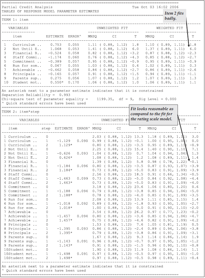
Figure 2.26: Response Model Parameter Estimates for the Partial Credit Model

2.3.3 Summary

In this section, ACER ConQuest has been used to fit partial credit and rating scale models. Some key points covered were:

The codes statement can be used to provide a list of valid codes.
The recode statement is used to change the codes that are given in the response block (defined in the format statement) for the data file.
The number of response categories modelled by ACER ConQuest for each item is the number of unique codes (after recoding) for that item.
Response categories and item scores are not the same thing.
The model statement can be used to fit different models to the same data.
The deviance statistic can be used to choose between models.

2.4 The Analysis of Rater Effects

The item response models, such as simple logistic, rating scale and partial credit, that have been illustrated in the previous two sections, assume that the observed responses result from the two-way interaction between the agents of measurement⁸ and the objects of measurement.⁹ With the increasing importance of performance assessment, Linacre (1994) recognised that the responses that are gathered in many contexts do not result from the interaction between an object and a single agent: the agent is often a composite of more fundamental subcomponents.¹⁰ Consider, for example, the assessment of writing, where a stimulus is presented to a student, the student prepares a piece of writing, and then a rater makes a judgment about the quality of the writing performance. Here, the object of measurement is clearly the student; but the agent is a combination of the rater who makes the judgment and the stimulus that serves as a prompt for the student’s writing. The response that is analysed by the item response model is influenced by the characteristics of the student, the characteristics of the stimulus, and the characteristics of the rater. Linacre (1994) would label this a three-faceted measurement context, the three facets being the student, the stimulus and the rater.

Using an extension of the partial credit model to this multifaceted context, Linacre (1994) and others have shown that item response models can be used to identify raters who are harsher or more lenient than others, who exhibit different patterns in the way they use rating schemes, and who make judgments that are inconsistent with judgments made by other raters. This section describes how ACER ConQuest can fit a multifaceted measurement model to analyse the characteristics of a set of 16 raters who have rated a set of writing tasks using two criteria.

2.4.1 a) Fitting a Multifaceted Model

2.4.1.1 Required files

The data that we are analysing are the ratings of 8296 Year 6 students’ responses to a single writing task. The data were gathered as part of a study reported in Congdon & McQueen (1997). Each of the 8296 students’ writing scripts was graded by two raters, randomly chosen from a set of 16 raters; and the second rating for each script was performed blind. The random allocation of scripts to the raters, in conjunction with the very large number of scripts, resulted in links between all raters being obtained. When assessing the scripts, each rater was required to provide two ratings, one labelled OP (overall performance) and the other TF (textual features).¹¹ The rating of both the OP and TF was undertaken against a sixpoint scale, with the labels G, H, I, J, K and L used to indicate successively superior levels of performance. For a small number of scripts, ratings of this nature could not be made; and the code N was used to indicate this occurrence.

The files used in this sample analysis are:

filename	content
ex3a.cqc	The command statements.
ex3_dat.txt	The data.
ex3a_shw.txt	The results of the multifaceted analysis.
ex3a_itn.txt	The results of the traditional item analyses.

(The last two files are created when the command file is executed.)

The data were entered into the file ex3_dat.txt, using one line per student. Rater identifiers (of two characters in width) for the first and second raters who rated the writing of each student are entered in columns 17 and 18 and columns 19 and 20, respectively. Each of the two raters produced an OP and a TF rating for the script. The OP and TF ratings made by the first rater have been entered in columns 21 and 22, and the OP and TF ratings made by the second rater have been entered in columns 25 and 26.

2.4.1.2 Syntax

ex3a.cqc is the command file used in this tutorial for fitting one possible multifaceted model to the data outlined above. The command file is shown in the code box below, and the list underneath the code box analyzes each line of syntax.

ex3a.cqc:

Title Rater Effects Model One;
datafile ex3_dat.txt;
format rater 17-18 rater 19-20 
       responses 21-22 responses 25-26 ! criteria(2);
codes G,H,I,J,K,L;
score (G,H,I,J,K,L) (0,1,2,3,4,5);
labels 1 OP !criteria;
labels 2 TF !criteria;
model rater + criteria + step;
estimate!nodes=20;
show !estimates=latent >> results/ex3a_shw.txt;
itanal >> results/ex3a_itn.txt;

Line 1
Gives a title for the analysis. The text supplied after the title command will appear on the top of any printed ACER ConQuest output.
Line 2
Indicates the name and location of the data file.
Lines 3-4
Multifaceted data can be entered into data sets in many ways. Here, two sets of ratings for each student have been included on each line in the data file, and explicit rater codes have been used to identify the raters. For each of the raters, there is a matching pair of ratings (one for OP and one for TF). The OP and TF ratings are implicitly identified by the columns in which the data are entered. The ACER ConQuest format statement is very flexible and can cater for many alternative data specifications. In this format statement, you will notice that rater is used twice. The first use indicates the column location of the rater code for the first rater, and the second use indicates the column location of the rater code for the second rater. This is followed by two variables indicating the location of the responses (referred to as response blocks). Each response block is two characters wide; and since the default width of a response is one column, each response block refers to two responses, an OP and a TF rating. The first response block (columns 21 and 22) will be associated with the first rater, and the second response block (columns 25 and 26) will be associated with the second rater.

This format statement also includes an option, criteria(2), which assigns the variable name criteria to the two responses that are implicitly identified by each response block. If this option had been omitted, the default variable name for the responses would be item.

This format statement spans two lines in the command file. Command statements can be 1023 characters in length and can cover any number of lines in a command file. The semi-colon (;) is the separator between statements, not the return or new line characters.
Line 5
The codes statement restricts the list of valid response codes to G, H, I, J, K, and L. All other responses will be treated as missing-response data.
Line 6
The score statement assigns score levels to each of the response categories. Here, the left side of the score argument shows the six valid codes defined by the codes statement, and the right side gives six matching scores. The six distinct codes on the left indicate that the item response model will model six categories for each item; the scores on the right are the scores that will be assigned to each category.

NOTE: As discussed in the previous section, ACER ConQuest makes an important distinction between response categories and response levels (or scores). The number of item response categories that will be modelled by ACER ConQuest is determined by the number of unique codes that exist after all recodes have been performed. ACER ConQuest requires a score for each response category. This can be provided via the score statement. Alternatively, if the score statement is omitted, ACER ConQuest will treat the recoded responses as numerical values and use them as scores. If the recoded responses are not numerical values, an error will be reported.
Lines 7-8
In the previous sample analyses, variable labels were read from a file. Here the criteria facet contains only two levels (the OP and TF ratings), so the labels are given in the command file using labels command syntax. These labels statements have two arguments. The first argument indicates the level of the facet to which the label is to be assigned, and the second argument is the label for that level. The option gives the facet to which the label is being applied.
Line 9
The model statement here contains three terms; rater, criteria and step. This model statement indicates that the responses are to be modelled with three sets of parameters: a set of rater harshness parameters, a set of criteria difficulty parameters, and a set of parameters to describe the step structure of the responses.

EXTENSION: The model statement in this sample analysis includes main effects only. An interaction term rater*criteria could be added to model variation in the difficulty of the criteria across the raters. Similarly, the model specifies a single step-structure for all rater and criteria combinations. Step structures that were common across the criteria but varied with raters could be modelled by using the term rater*step, step structures that were common across the raters but varied with criteria could be modelled by using the term criteria*step, and step structures that varied with rater and criteria combinations could be modelled by using the term rater*criteria*step.
Line 10
The estimate statement initiates the estimation of the item response model.
Line 11
The show statement produces a display of the item response model parameter estimates and saves them to the file ex3a_shw.txt. The option estimates=latent requests that the displays include an illustration of the latent ability distribution.
Line 12
The itanal statement produces a display of the results of a traditional item analysis. As with the show statement, we have redirected the results to a file (in this case, ex3a_itn.txt).

2.4.1.3 Running the Multifaceted Sample Analysis

To run this sample analysis, start the GUI version of ACER ConQuest and open the control file ex3a.cqc.

Select Run\(\rightarrow\)Run All. ACER ConQuest will begin executing the statements that are in the file ex3a.cqc; and as they are executed, they will be echoed on the screen. When ACER ConQuest reaches the estimate statement, it will begin fitting the multifaceted model to the data; and as it does, it will report on the progress of this estimation. Due to the large size of this data file, ACER ConQuest will take some time to perform this analysis. During estimation, ACER ConQuest reports a warning message:

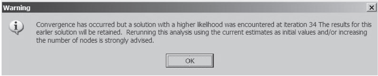
As the scores of the writing test spread students far apart, as indicated by the estimated variance of the ability distribution (5.7 logits), this suggests that more nodes to cover the ability range are required in the estimation process.

To re-run ACER ConQuest with more nodes during the estimation, modify the estimate command as follows:

Line 10
estimate ! nodes=30;

The default number of nodes is 15. The above estimate command requests ACER ConQuest to use 30 nodes to cover the ability range.

Re-run ACER ConQuest by selecting Run\(\rightarrow\)Run All from the menu. This time, ACER ConQuest no longer reports a warning for convergence problems.

After the estimation is complete, the two statements that produce output (show and itanal) will be processed. The results of the show statement can be found in the file ex3a_shw.txt, and the results of the itanal statement can be found in the file ex3a_itn.txt. On this occasion, the show statement will produce six tables.

From Figure 2.27, we note that there were 16 raters and that the harshness ranges from a high of 0.977 logits for rater 14 (the first rater in the table) to a low of –1.292 for rater 19 (the fourth rater in the table). This is a range of 2.123, which appears quite large when compared to the standard deviation of the latent distribution, which is estimated to be 2.37 (the square root of the variance that is reported in the third table (the population model) in ex3a_shw.txt). That means that ignoring the influence of the harshness of the raters may move a student’s ability estimate by as much as one standard deviation of the latent distribution. We also note that, with this model, the raters do not fit particularly well. The high mean squares (and corresponding positive t values) suggest quite a bit of unmodelled noise in the ratings.

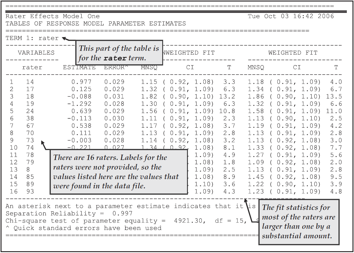
Figure 2.27: Parameter Estimates for Rater Harshness

In Figure 2.28, we note that the OP and TF difficulty estimates are very similar, differing by just 0.178 logits. This difference is significant but very small. The mean square fit statistics are less than one, suggesting that the criteria could have unmodelled dependency.

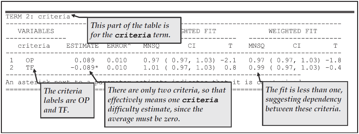
Figure 2.28: Parameter Estimates for the Criteria

Figure 2.29 shows the step parameter estimates. The fit here is not very good, particularly for steps 1 and 4, suggesting that we should model step structures that interact with the facets. It is pleasing to note that the estimates for the steps themselves are ordered and well separated.

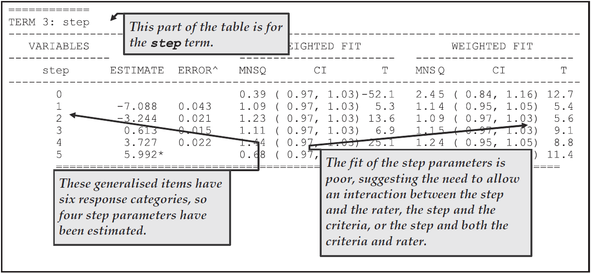
Figure 2.29: Parameter Estimates for the Steps

Figure 2.30 is the map of the parameter estimates that is provided in ex3a_shw.txt. The map shows how the variation between raters in their harshness is large relative to the difference in the difficulty of the two tasks. It also shows that the rater harshness estimates are well centred for the estimated ability distribution.

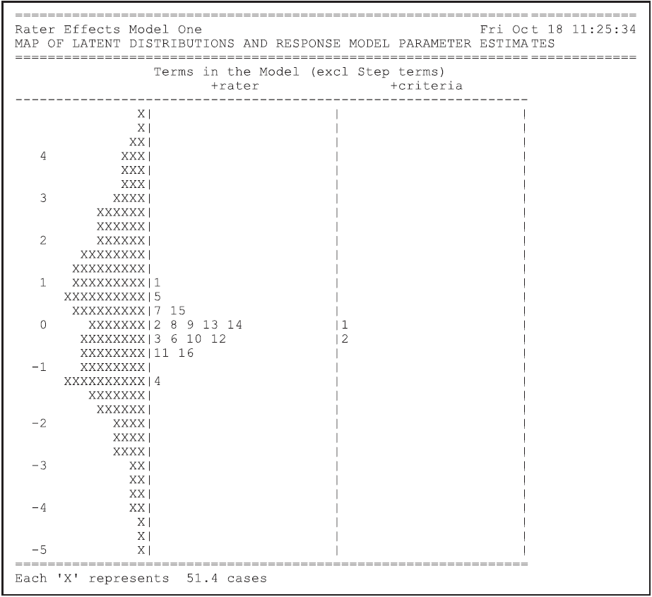
Figure 2.30: Map of the Parameter Estimates for the Multifaceted Model

The file ex3a_itn.txt contains basic traditional statistics for this multifaceted analysis, extracts of which are shown in Figures 2.31 and 2.32.

In this analysis, the combination of the 16 raters and two criteria leads to 32 generalised items.¹² The statistics for each of these generalised items is reported in the file ex3a_itn.txt.

Figure 2.31 shows the statistics for the last generalised item, which is the combination of rater 93 (the sixteenth rater) and criterion TF (the second criterion). For this generalised item, the total number of students rated by this rater on this criteria is shown (in this case, 1002); and an index of discrimination (the correlation between students’ scores on this item and their total score) is shown (in this case, 0.87). This discrimination index is very high, but it should be interpreted with care since only four generalised items are used to construct scores for each student. Thus, a student’s score on this generalised item contributes 25% to their total score.

For each response category of this generalised item, the number of observed responses is reported, both as a count and as a percentage of the total number of responses to this generalised item. The point-biserial correlations that are reported for each category are computed by constructing a set of dichotomous indicator variables, one for each category. If a student’s response is allocated to a category for an item, then the indicator variable for that category will be coded to 1; if the student’s response is not in that category, it will be coded to 0. The point biserial is then the correlation between the indicator variable and the student’s total score. It is desirable for the point biserials to be ordered in a fashion that is consistent with the category scores. However, sometimes point biserials are not ordered when a very small or a very large proportion of the item responses are in one category. This can be seen in Figure 2.31, where only seven of the 1002 cases have responses in category G.

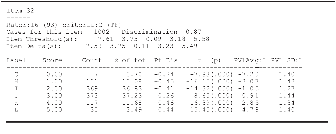
Figure 2.31: Extract from the Item Analysis for the Multifaceted Analysis

The itanal statement’s output concludes with a set of summary statistics (Figure 2.32). For the mean, standard deviation, variance and standard error of the mean, the scores have been scaled up so that they are reported on a scale consistent with students responding to all of the generalised items.

NOTE: Traditional methods are not well suited to multifaceted measurement. If more than 10% of the response data is missing — either at random or by design (as will often be the case in multifaceted designs) — the test reliability and standard error of measurement will not be computed.

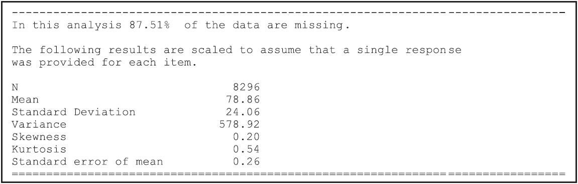
Figure 2.32: Summary Statistics for the Multifaceted Analysis

2.4.2 b) The Multifaceted Analysis Restricted to One Criterion

In analysing these data with the multifaceted model, the fit statistics have suggested a lack of independence between the raters’ judgments for the two criteria and evidence of unmodelled noise in the raters’ behaviour. Here, therefore, an additional analysis is undertaken that adds some support to the hypothesis that the raters’ OP and TF judgments are not independent. In this second analysis, only one criterion (OP) is analysed.

2.4.2.1 Required files

The files that we use in this sample analysis are:

filename	content
ex3b.cqc	The command statements.
ex3_dat.txt	The data.
ex3b_shw.txt	The results of the single-criterion multifaceted analysis.

(The last file is created when the command file is executed.)

2.4.2.2 Syntax

ex3b.cqc is the command file used in this tutorial for fitting the multifaceted model to our data, but using only one of the criteria. The code listed here is very similar to ex3a.cqc, the command file from the previous analysis (as shown in section 2.4.1.2). So only the differences will be discussed in the list underneath the code box.

ex3b.cqc:

Title Rater Effects Model Two;
datafile ex3_dat.txt;
format rater 17-18 rater 19-20 
       responses 21 responses 25 ! criteria(1);
codes G,H,I,J,K,L;
score (G,H,I,J,K,L) (0,1,2,3,4,5);
labels 1 OP !criteria;
/*labels 2 TF !criteria;*/
model rater + criteria + step;
estimate !nodes=20;
show ! estimates=latent >> Results/ex3b_shw.txt;

Lines 1-2
As in the command file of the previous analysis, ex3b.cqc.
Line 3-4
The response blocks in the format statement now refer to one column only, the column that contains the OP criteria for each rater. Note that in the option we now indicate that there is just one criterion in each response block.
Lines 5-7
As in the command file of the previous analysis, ex3b.cqc.
Line 8
The labels statement for the TF criterion is now unnecessary, so we have enclosed it inside comment markers (/* and */).
Lines 9-11
As for lines 9, 10, and 11 in ex3a.cqc, except the show statement output is directed to a different file, ex3b_shw.txt.

2.4.2.3 Running the Multifaceted Model for One Criterion

To run this sample analysis, start the GUI version of ACER ConQuest and open the control file ex3b.cqc.

Select Run\(\rightarrow\)Run All.

ACER ConQuest will begin executing the statements that are in the file ex3b.cqc; and as they are executed, they will be echoed on the screen. When ACER ConQuest reaches the estimate statement, it will begin fitting the multifaceted model to the data; and as it does so, it will report on the progress of the estimation. Due to the large size of this data file, ACER ConQuest will take some time to perform this analysis.

In Figures 2.33 and 2.34, the rater and step parameter estimates are given for this model from the second table in the file ex3b_shw.txt. The part of the table that reports on the criteria facet is not shown here, since there is only one criterion and it must therefore have an estimate of zero. In fact, the inclusion of the criteria term in the model statement was redundant.

A comparison of Figures 2.33 and 2.34 with Figures 2.27, 2.28, and 2.29 shows that this second model leads to an improved fit for both the rater and step parameters. It would appear that the apparent noisy behaviour of the raters, as illustrated in Figure 2.27, is a result of the redundancy in the two criteria and is not evident if a single criterion is analysed. The fit statistics for the steps are similarly improved, suggesting either that the redundancy between the criteria was influencing the step fits or that there is a rater by criteria interaction.

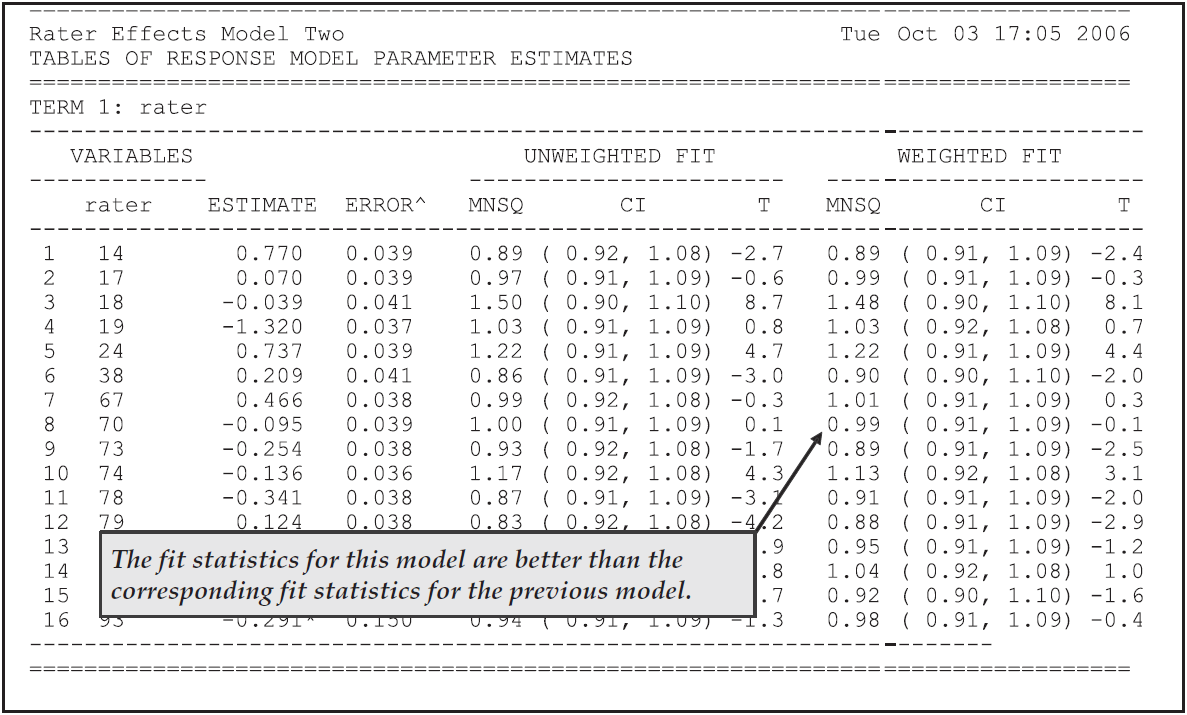
Figure 2.33: Rater Harshness Parameter Estimates

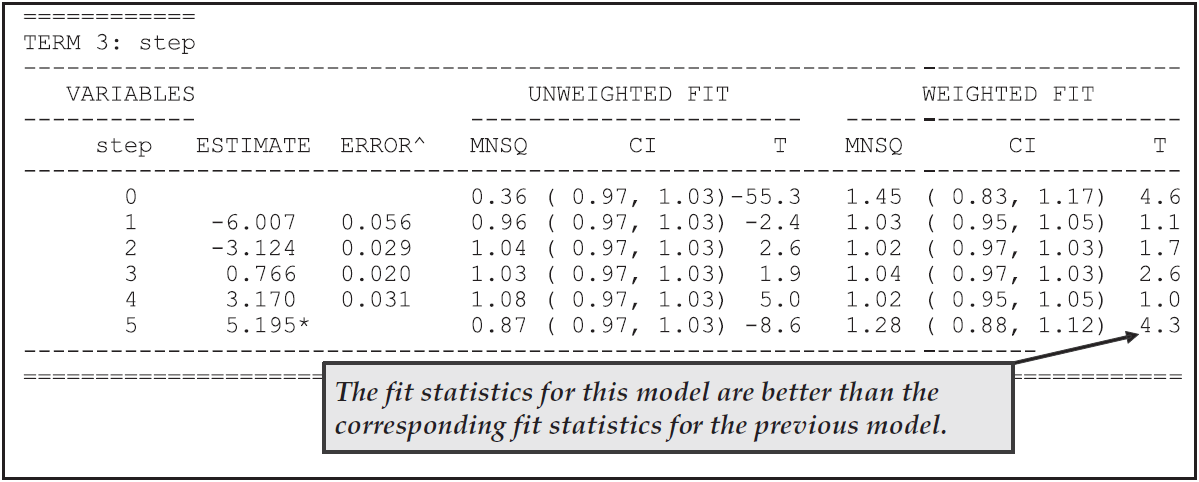
Figure 2.34: Step Parameter Estimates

The dependency possibility can be further explored by using the model that assumed independence (the first sample analysis in this section) to calculate the expected frequencies of various pairs of OP and TF ratings and then comparing the expected frequencies with the observed frequencies of those pairs. Figure 2.35 shows a two-dimensional frequency plot of the observed and expected number of scores for pairs of values of TF and OP given by rater 85. The diagonal line shows the points where the TF and OP scores are equal. It is noted that the observed frequencies are much higher than the expected frequencies along this diagonal, indicating that rater 85 tends to give more identical scores for TF and OP than one would expect. Similar patterns are also observed for other raters. It appears that a model that takes account of the severity of the rater and the difficulty of the criteria does not fit these data well.

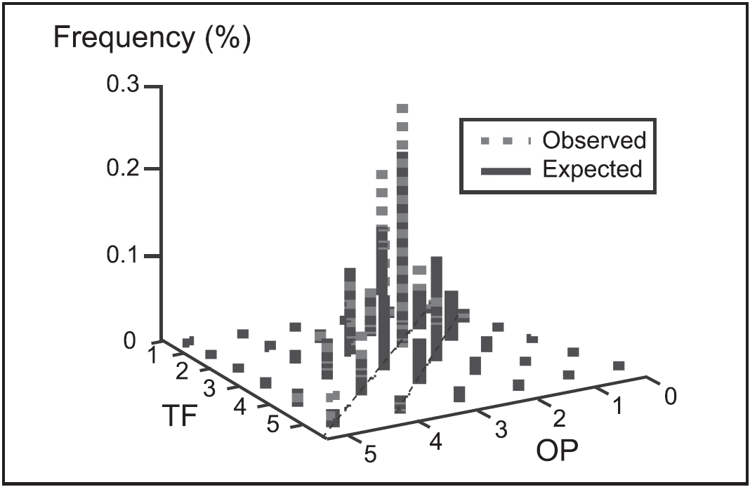
Figure 2.35: Observed Versus Expected Frequencies for Pairs of OP and TF Scores

WARNING: In section 2.3, the deviance statistic was used to compare the fit of a rating scale and partial credit model. It is not appropriate to use the deviance statistic to compare the fit of the two models fitted in this section. The deviance statistic can only be used when one model is a submodel of the other. For this to occur, the models must result in response patterns that are the same length, and each of the items must have the same number of response categories in each of the analyses (which was not the case here).

2.4.3 Summary

In this section, we have seen how to fit multifaceted models with ACER ConQuest. Our sample analysis has used only one additional facet (rater), but ACER ConQuest can analyse up to 50 facets.

Some key points we have covered in this section are:

ACER ConQuest can be used to fit multifaceted item response models easily.
The format statement is very flexible and can deal with many of the alternative ways that multifaceted data can be formatted (see the command reference in Section 4 for more examples).
A score statement can be used to assign scores to the response categories that are modelled.
We have reiterated the point that response categories and item scores are not the same thing.
Fit statistics can be used to suggest alternative models that might be fitted to the data.

2.5 Many Facets and Hierarchical Model Testing

In section 2.4, the notion of additional measurement facets is introduced, and data was analysed with one additional facet, a rater facet. The number of facets that can be used with multifaceted measurement models is theoretically unlimited, although, as shall be seen in this section, the addition of each new facet adds considerably to the range of models that need to be considered.¹³ A number of techniques are available for choosing between alternative models for multifaceted data. First, the deviance statistic of alternative models can be compared to provide a formal statistical test of the relative fit of models. Second, the fit statistics for the parameter estimates can be used, as was done in the previous section. Third, the estimated values of the parameters associated with a term in a model can be examined to see if that term is necessary. In this section, we illustrate these strategies for choosing between the many alternative multifaceted models that can be applied to data that have more than two facets.

The data that we are analysing in this section are simulated three-faceted data.¹⁴ The data were simulated to reflect an assessment context in which 500 students have each provided written responses to two out of a total of four writing topics. Each of these tasks was then rated by two out of four raters against five assessment criteria. For each of the five criteria, a four-point rating scale was used with codes 0, 1, 2 and 3. This results in four sets of ratings (two essay topics by two raters’ judgments) against the five criteria for each of the 500 students. In generating the data, two raters and two topics were randomly assigned to the students, and the model used assumed that the raters differed in harshness, that the criteria differed in difficulty, and that the rating structure varied across the criteria. The topics were assumed to be of equal difficulty; there were no interactions between the topic, criteria and rater facets; and the step structure did not vary with rater or topic.

The files used in this sample analysis are:

filename	content
ex4a.cqc	The command statements used for the first analysis.
ex4_dat.txt	The data.
ex4_lab.txt	The variable labels for the facet elements.
ex4a_prm.txt	Initial values for the item parameter estimates.
ex4a_reg.txt	Initial values for the regression parameter estimates.
ex4a_cov.txt	Initial values for the variance parameter estimates.
ex4a_shw.txt	Selected results of the first analysis.
ex4b.cqc	The command statements used for the second analysis.
ex4b_1_shw.txt and ex4b_2_shw.txt	Selected results of the second analysis.
ex4c.R	The R command file used for the third analysis.
ex4c.cqc	The ACER ConQuest command statements used for the third analysis.
ex4c_1_shw.txt through ex4c_11_shw.txt	Selected results of the third analysis.

(The _prm.txt, _reg.txt, _cov.txt, and _shw.txt files are created when the command file is executed.)

The data were entered into the file ex4_dat.txt using four lines per student, one for each rater and topic combination. For each of the lines, column 1 contains a rater code, column 3 contains a topic code and columns 5 through 9 contain the ratings of the five criteria given by the matching rater and topic combination.

2.5.1 a) Fitting a General Three-Faceted Model

In the first analysis, we fit a model that assumes main effects for all facets, the set of three two-way interactions, and a step structure that varies with topic, item and rater.

2.5.1.1 Syntax

ex4a.cqc is the command file used in the first analysis to fit one possible multifaceted model to these data. The code box below shows the contents of the file, and the list underneath the code box explains each line of syntax.

ex4a.cqc:

datafile ex4_dat.txt;
format rater 1 topic 3 responses 5-9 /
       rater 1 topic 3 responses 5-9 /
       rater 1 topic 3 responses 5-9 /
       rater 1 topic 3 responses 5-9 ! criteria(5);
label << ex4_lab.txt;
set update=yes,warning=no;
model   rater + topic + criteria + rater*topic + rater*criteria +
        topic*criteria + rater*topic*criteria*step;     
export parameters >> Results/ex4a_prm.txt;
export reg >> Results/ex4a_reg.txt;
export cov >> Results/ex4a_cov.txt;
estimate ! nodes=10, stderr=empirical;
show parameters !estimates=latent,tables=1:2:4>> Results/ex4a_shw.txt;

Line 1
Indicates the name and location of the data file.
Lines 2-5
Multifaceted data can be entered into data sets in many ways. The ACER ConQuest format statement is very flexible and can cater for many alternative data specifications. Here the data are spread over four lines for each student. Each line contains a rater code, a topic code and five responses. The slash (/) character is used to indicate that the following data should be read from the next line of the data file. The multiple use of the terms rater, topic and responses allows us to read the multiple sets of ratings for each student. In this case, the term rater is used four times, topic four times and responses four times. Thus, the rater and topic indicated on the first line for each case will be associated with the responses on the first line, the rater and topic on the second line will be associated with the responses on the second line, and so on. More generally, if variables are repeated in a format statement, the n-th occurrence of responses will be associated with the n-th occurrence of any other variable, or the n-th occurrence of responses will be matched with the highest occurrence of any other variable if n is greater than the number of occurrences of that variable.

This format statement also includes an option, criteria(5), which assigns the variable name criteria to the five responses that are implicitly identified by the response block. If this option had been omitted, the default variable name for the responses would have been item.
Line 6
The labels for the facets in this analysis are to be read from the file ex4_lab.txt. The contents of this file are shown in Figure 2.36. Here we have provided labels for each of the three facets. The character string ===> precedes the name of the facet, and the following lines contain the facet level and then the label that is to be assigned to that level.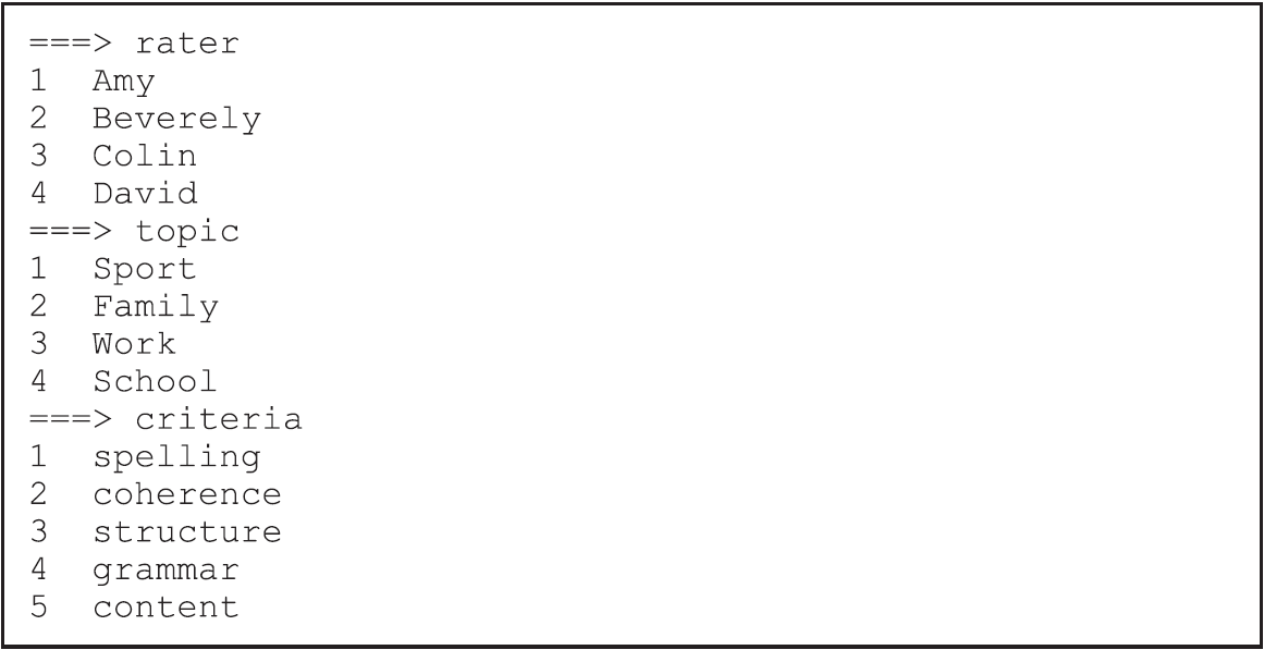

Figure 2.36: The Labels File for the Many Facets Sample Analysis
Line 7
The set statement can be used to alter some of ACER ConQuest’s default values. In this case, the default status of the update and warnings settings has been changed. When update is set to yes, in conjunction with the following export statements, updated parameter estimates will be written to a file at the completion of every iteration. This option is particularly valuable when analyses take a long time to execute. If the update option is set to yes and you have to terminate the analysis for some reason (e.g., you want to use the computer for something else and ACER ConQuest is monopolising CPU time), you can interrupt the job and then restart it at some later stage with starting values set to the most recent parameter estimates. (To use these starting values, you would have to add one or more import statements to the command file.) Setting warnings to no tells ACER ConQuest not to report warning messages. Errors, however, will still be reported. Setting warnings to no is typically used in conjunction with setting update to yes in order to suppress the warning message that there is a file overwrite at every iteration.
Lines 8-9
The model statement contains seven terms: rater, topic, criteria, rater*topic, rater*criteria, topic*criteria, and rater*topic*criteria*step. This model statement indicates that seven sets of parameters are to be estimated. The first three are main effects and correspond to a set of rater harshness parameters, a set of topic difficulty parameters, and a set of criteria difficulty parameters. The next three are two-way interactions between the facets. The first of these interaction terms models a variation in rater harshness across the topics (or, equivalently, variation in topic difficulty across the raters), the second models a variation in rater harshness across the criteria, and the third represents a variation in the topic difficulties across the criteria. The final term represents a set of parameters to describe the step structure of the responses. The step structure is modelled as varying across all combinations of raters, topics and criteria.

One additional term could be added to this model: the three-way interaction between raters, topics and criteria.
Lines 10-12
The export statements request that the parameter estimates be written to text files in a simple, unlabelled format. The export statement can be used to produce files that are more readily read by other software. Further, the format of each export file matches the format of ACER ConQuest import files so that export files that are written by ACER ConQuest can be re-read as either anchor files or initial value files.¹⁵
Line 13
The estimate statement initiates the estimation of the item response model. In this case, two options are used to change the default settings of the estimation procedures. The nodes=10 option means that the numerical integration that is necessary in the estimation will be done with a Gauss-hermite quadrature method using 10 nodes.¹⁶ The default number of nodes is 15, but we have chosen to reduce the number of nodes to 10 for this sample analysis, since it will reduce the processing time. Simulation results by Wu & Adams (1993) illustrate that 10 nodes will normally be sufficient for accurate estimation. The stderr=empirical option causes ACER ConQuest to compute the full error variance-covariance matrix for the model that has been estimated. This method provides the most accurate estimates of the asymptotic error variances that ACER ConQuest can compute. It does, however, take a considerable amount of computing time, even on very fast machines. In Estimating Standard Errors in Chapter 3, we discuss the circumstances under which it is desirable to use the stderr=empirical option. In this case, we have used it because of the large number of facets, each of which has only a couple of levels.
Line 14
The show statement produces a display of the item response model parameter estimates and saves them to the file ex4a_shw.txt. The option estimates=latent requests that the displays include an illustration of the latent ability distribution. The option tables=1:2:4 limits the output to tables 1, 2 and 4.

2.5.1.2 Running the Multifaceted Sample Analysis

To run this sample analysis, start the GUI version of ACER ConQuest and open the control file ex4a.cqc.

Select Run\(\rightarrow\)Run All. ACER ConQuest will begin executing the statements that are in the file ex4a.cqc; and as they are executed, they will be echoed in the Output window. When ACER ConQuest reaches the estimate statement, it will begin fitting the multifaceted model to the data; and as it does so, it will report on the progress of this estimation. This analysis will take around 700 iterations to converge, and the calculation of the standard errors may take a considerable amount of time. After the estimation is complete, the output from the show statement can be found in the file ex4a_shw.txt. Figures 2.37 and 2.38 are extracts from the second table in this file.

Figure 2.37 shows the parameter estimates for the three main effects: rater, topic and criteria. Notice that the separation reliability for the topic is close to zero and that the variation between the topic parameter estimates is not significant. This result suggests that the topic term might be deleted from the model because the topics do not vary in their difficulty. (Thus, ACER ConQuest has confirmed the model we used in our data simulation.)

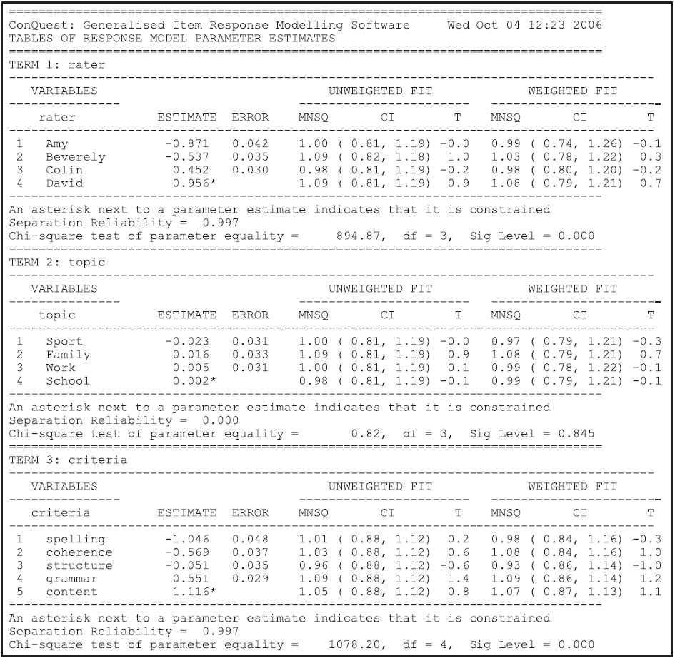
Figure 2.37: The Parameter Estimates for Rater Harshness, Topic Difficulty and Criterion Difficulty

Figure 2.38 shows the parameter estimates for one of the three two-way interaction terms. The results reported in this figure suggest that there is no interaction between the topic and criteria. (Again, ACER ConQuest has confirmed the model we used in our data simulation.) The results for the two remaining two-way interaction terms are not reported here; however, if you examine them in the file ex4a_shw.txt you will see that, although the effects are statistically significant, they are very small and we could probably ignore them.

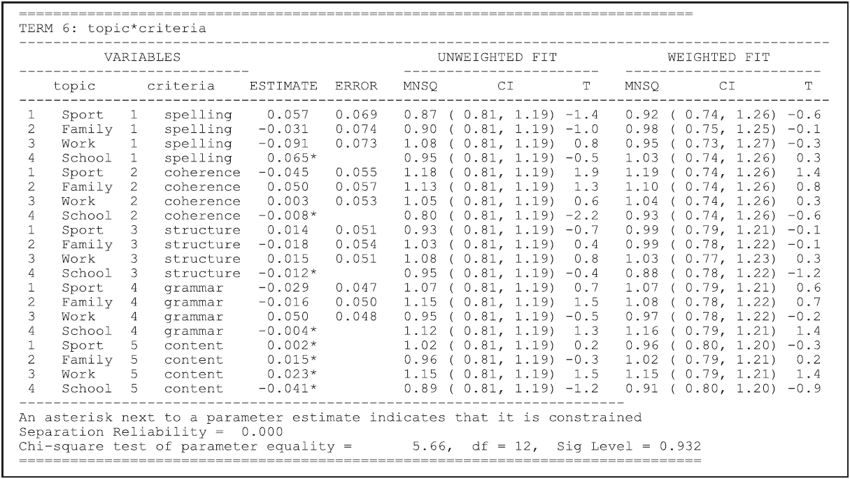
Figure 2.38: Parameter Estimates for the topic*criteria Interaction

2.5.2 b) The Fit of Two Additional Alternative Models

Many submodels of the model analysed with the command file in Figure ex4a.cqc (discussed in Section 2.5.1.1) can be fitted to these data. As we mentioned above, the model that was actually used in the generation of these data can be fitted by replacing the model statement in ex4a.cqc with model rater + criteria + criteria*step.

The file ex4b.cqc contains statements that will fit this submodel and an even simpler model (rater + step). The item response model parameter estimates that are obtained from the first of these models are saved to the file ex4b_1_shw.txt and shown in Figure 2.39. As would be expected, the fit for each of the parameters is good.

The other important thing to note about Figure 2.39 is the values of the parameter estimates. When the data in ex4_dat.txt were generated, the rater parameters were set at –1.0, –0.5, 0.5 and 1.0 and the criteria parameters were set at –1.2, –0.6, 0, 0.6 and 1.2.

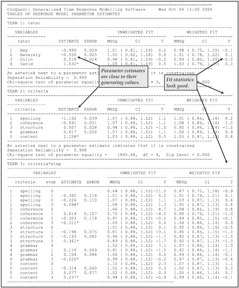
Figure 2.39: Parameter Estimates for model rater + criteria + criteria*step;

Figure 2.40, an excerpt of ex4b_2_shw.txt, shows the item parameter estimates when the model statement is changed to model rater + step, which assumes that there is no variation between the criteria in difficulty, a simplification that we know does not hold for these data. The fact that this model is not appropriate for the data can be easily identified by the fact that the deviance has increased significantly from the deviance for the model that was fit in Figure 2.39 (as shown in the first table generated by the show statement). This observation is discussed in detail in the next section, A Sequence of Models. From Figure 2.40, however, we note that the fit statistics, at least in the case of the rater parameters, are smaller than they should be.

When lower than expected fit statistic values are found, it is generally a result of unmodelled dependencies in the data. In the previous section, we saw that low fit was probably due to an unmodelled dependency between the two criteria, OP and TF. Here the low fit suggests that there is an unmodelled consistency between the rater judgments. The judgments across raters are more consistent than the model expects, and this has arisen because an element of consistency between judgments in the ratings can be traced to the variance in the criteria difficulties, a variation that is not currently being modelled.

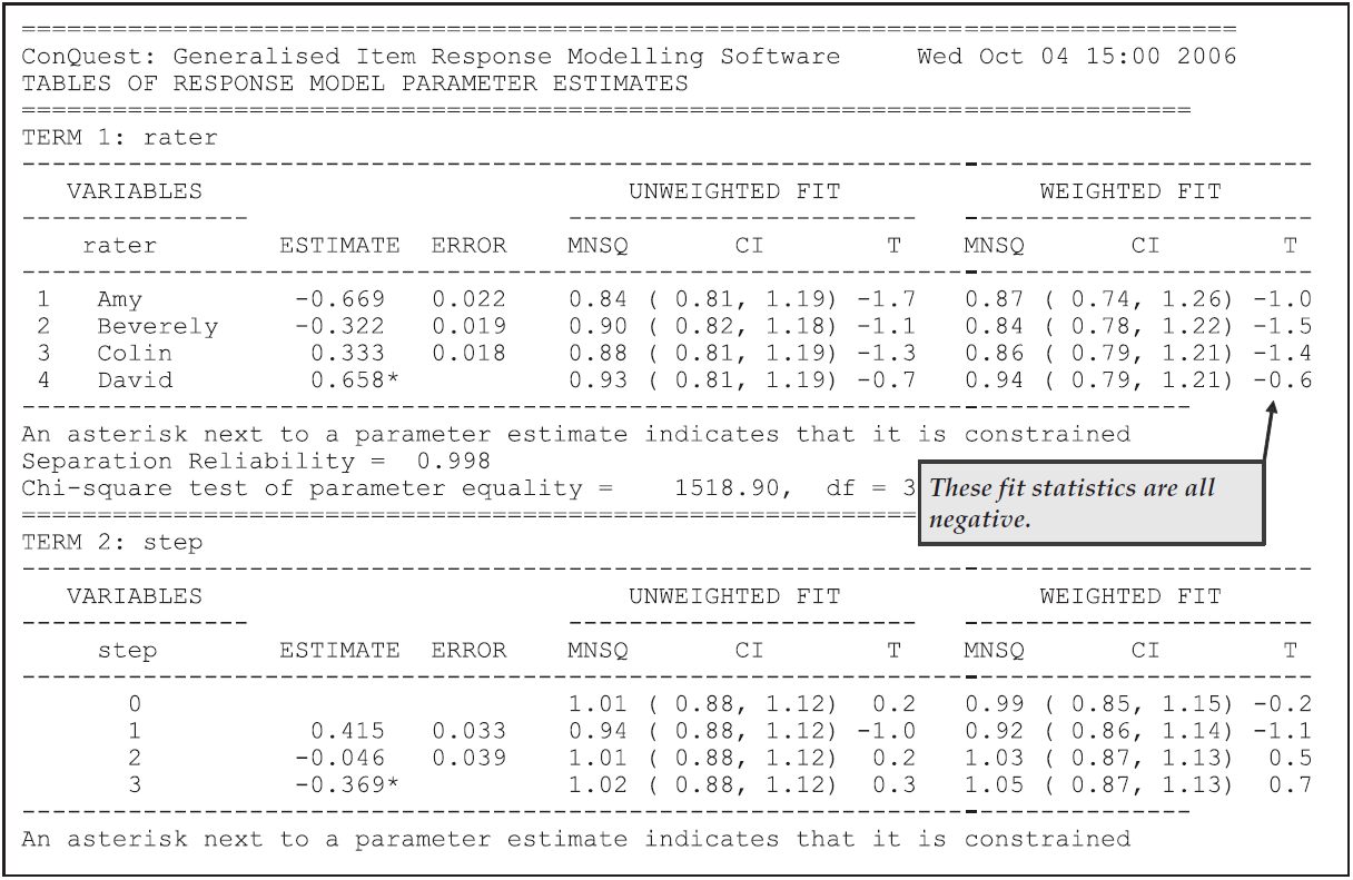
Figure 2.40: Parameter Estimates for model rater + step;

2.5.3 c) A Sequence of Models

A search for a model that provides the most parsimonious fit to these data can be undertaken in a systematic fashion by using hierarchical model fitting techniques in conjunction with the use of the Chi-squared test of parameter equality.

2.5.3.1 Syntax

We will fit the models in the hierarchy shown in Figure 2.41 using R in conjunction with conquestr. The R command file used is ex4c.R. Since we are only interested in the effect of using different terms in the model, all other aspects of the command file, i.e. the format of our data and the method of estimation, stay the same across all models in the hierarchy. The use of R will allow us to efficiently loop through all models of interest, by only updating/overwriting the model statement in the command file ex4c.cqc at each iteration. At the end of each iteration (i.e. after each model has been fitted) we retain the statistics of interest: Deviance and the number of parameters. These will allow us to conduct a Chi-squared test between nested models in the hierarchy, and hence decide which terms are significant.

2.5.3.2 Results

The results of all 11 fitted models are written to the files ex4c_1_shw.txt through ex4c_11_shw.txt. A summary of Deviance statistics is written to the csv file ex4cDeviances.csv. Figure 2.41 illustrates the hierarchy of models that are included in ex4c.R and summarises the fit of the models.

We can now use the Chi-squared statistics to compare any pair of nested models. Under the null hypothesis that the nested/smaller model is correct (rather than the model with more parameters), the Chi-squared statistic is distributed according to a Chi-squared distribution with degrees of freedom given by the difference in number of parameters between the two models.

Notice, as we move through the hierarchy from model (1) to model (5) and then model (9), how the fit is not significantly worsened by removing terms. This is evident in the Chi-squared statistics being relatively close to their null means (i.e. their hypothesised degrees of freedom). It may be worth to note that some of the p-values along this path are between 0.01 and 0.05, and hence fall below the common significance threshold 0.05. For example, moving from model (2) to (3) yields \(P(\chi^2_{33}>53.5)=0.013\). However, in the interest of finding a parsimonious model one may want to adapt a stricter threshold than 0.05.

By similar reasoning, model fit does not worsen significantly following the path (1) to (3) and then (7) to (9).

Towards the bottom of the hierarchy we then encounter models which do not explain sufficient variability in the data at even the lowest signifcance levels. Here the Chi-squared statistics and their null means differ by orders of magnitude:

Comparing models (5) and (6) (\(\chi^2\)=1578.5, df=3), we note that the rater term is necessary—that is, there is significant variation between the raters in their harshness.
Comparing models (9) and (10) (\(\chi^2\)=172.6, df=8), we can see that the step parameters vary significantly with criteria.

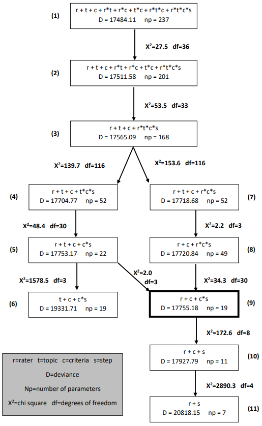
Figure 2.41: A Hierarchy of Models and Their Fit

2.5.4 Summary

In this section, we have seen how ACER ConQuest can be used to compare the fit of competing models that may be considered appropriate for a data set. We have seen how to use the deviance statistics, fit statistics and test of parameter equality to assist in the choice of a best fitting model.

2.6 Unidimensional Latent Regression

The term latent regression refers to the direct estimation of regression models from item response data. To illustrate the use of latent regression, consider the following typical situation. There are two groups of students, group A and group B, and it is of interest to estimate the difference in the mean achievement of the two groups. A common approach is to administer a test to the students and then use this test to produce achievement scores for all of the students. A standard procedure can then be applied, such as regression (which, in this simple case, becomes identical to a t-test), to examine the difference in the means of the achievement scores. Depending upon the model that is used to produce ‘student scores,’ this approach can result in misleading inferences about the differences in the means. Using the latent regression methods described by Adams, Wilson, & Wu (1997), ACER ConQuest avoids such problems by directly estimating the difference in the mean achievement of the groups from the item response data without first producing individual student scores.

The data used here are a subset of the data that were collected by Lokan, Lokan et al. (1996) as part of the Third International Mathematics and Science Study (TIMSS) (Beaton et al., 1996). The TIMSS data that we will be using are the mathematics achievement test data, collected from a sample of 6800 students in their first two years of secondary schooling in Australia.¹⁷

The TIMSS study used a sophisticated test item rotation plan that enabled achievement data to be gathered on a total of 158 test items while restricting the testing time for any individual student to 90 minutes. Details on how this was achieved are described in Adams & Gonzales (1996). In this section, we will be using the data to examine grade differences and gender differences in students’ mathematics achievement as tested by the TIMSS tests.

The data set used in this sample analysis, ex5_dat.txt, contains 6800 lines of data, one line for each student that was tested. Columns 20 to 177 contain the item responses. The TIMSS tests consist of multiple choice, short answer and extended response questions. For the multiple choice items, the codes 1, 2, 3, 4 and 5 are used to indicate the response alternatives to the items. For the short answer and extended response items, the codes 0, 1, 2 and 3 are used to indicate the student’s score on the item. If an item was not presented to a student, the code . (a period) is used; if the student failed to attempt an item and that item is part of a block of non-attempts at the end of a test, then the code R is used. For all other non-attempts, the code M is used. The first 19 columns of the data set contain identification and demographic information. In this example, only the data in columns 17 through 19 are used. Column 17 contains the code 0 for male students and 1 for female students; column 18 contains the code 0 for lower grade (first year of secondary school) students and 1 for upper grade (second year of secondary school) students; and column 19 contains the product of columns 17 and 18, that is, it contains 1 for upper grade female students and 0 otherwise.

2.6.1 a) A Latent Variable t-Test

In the first sample analysis that uses these data, it is of interest to estimate the difference in achievement between the lower and upper grades. To illustrate the value of directly estimating the differences using latent regression, only the first six items are used. Later in the section, we will compare the results obtained from analysing only these six items with the results obtained from analysing all 158 items.

2.6.1.1 Required files

The files used in this first sample analysis are:

filename	content
ex5a.cqc	The command statements used for the first analysis.
ex5_dat.txt	The data.
ex5_lab.txt	The variable labels for the items.
ex5a_mle.txt	Maximum likelihood ability estimates for the students.
ex5a_eap.txt	Expected a-posterior ability estimates for the students.
ex5a_shw.txt	Selected results of the analysis.
ex5a_itn.txt	The results of the traditional item analyses.

(The last four files will be created when the command file is executed.)

2.6.1.2 Syntax

The command file used in this sample analysis for a Latent Variable t-Test (Six Items) is ex5a.cqc. It is shown in the code box below, and explained line-by-line in the list that follows the code.

ex5a.cqc:

datafile ex5_dat.txt;
title     Australian TIMSS Mathematics Data--First Six Items; 
format    gender 17 level 18 gbyl 19 responses 20-25;
labels  << ex5_lab.txt;
key  134423 ! 1;
regression level;
model item;
estimate !fit=no;
show cases ! estimate=mle >> Results/ex5a_mle.txt;
show cases ! estimate=eap >> Results/ex5a_eap.txt;
show ! tables=3 >> Results/ex5a_shw.txt;
itanal >> Results/ex5a_itn.txt;

Line 1
Indicates the name and location of the data file.
Line 2
Gives a title for this analysis. The text that is given after the command title will appear on the top of any printed output. If a title is not provided, the default, ConQuest: Generalised Item Response Modelling Software, will be used.
Line 3
The format statement describes the layout of the data in the file ex5_dat.txt. This format indicates that a code for gender is located in column 17, a code for level is located in column 18, column 19 contains the code for a variable we have called gbyl, and responses are to be read from columns 20 through 25. We have not given a name to the responses, so they will be referred to as item.
Line 4
A set of labels for the items are to be read from the file ex5_lab.txt.

NOTE: The file ex5_lab.txt contains labels for all 158 items. These are all read and held in memory by ACER ConQuest, even though we are only using the first six items in this analysis.
Line 5
The argument of the key statement identifies the correct response for each of the six multiple choice test items. In this case, the correct answer for item 1 is 1, the correct answer for item 2 is 3, the correct answer for item 3 is 4, and so on. The length of the key statement argument is six characters, which is the length of the response block given in the format statement. The key statement option indicates that each correct answer will be recoded to 1. By default, incorrect answers will be recoded to 0.

NOTE: These data contain three kinds of missing-response data. The codes for these missing-response data are . (a period), M, and R. In this analysis, ACER ConQuest will treat . as missing-response data, since it is one of the default missing-response codes. Those data coded M and R will be treated as incorrect, because these codes do not match the values in the key statement argument.
Line 6
The independent variables that we want to include as predictors of the latent variable are included as arguments in the regression statement. By including the variable level as the argument here, we are instructing ACER ConQuest to regress latent ability onto level; and in this case, since level is coded 0 (lower grade) and 1 (upper grade), ACER ConQuest will estimate the difference between the means of these two groups. The regression statement is used to describe the ACER ConQuest population model.
Line 7
The model statement here contains only the term item because we are dealing with single-faceted dichotomous data.
Line 8
The estimate statement is used to initiate the estimation of the model. The fit=no option is included because in this sample analysis we are not concerned with the item fit and it will save time if the fit statistics are not computed.

TIP: If you want to regress the latent variable onto a categorical variable, then the categorical variable must first be appropriately recoded. For example, dummy coding or contrast coding can be used. A variable used in regression must be a numerical value, not merely a label. For example, gender would normally be coded as 0 and 1 so that the estimated regression is the estimated difference between the group means. Remember that the specific interpretation of the latent regression parameters depends upon the coding scheme that you have chosen for the categorical variable.
Line 9
The show statement produces a display of the results from fitting the model. Here the cases argument is used to request a set of ability estimates for the students. The estimates=mle option indicates that maximum likelihood estimates of the ability are requested, and they are redirected to the file ex5a_mle.txt. When case estimates are requested, both the option indicating the type of estimate and redirection to a file are required.
Line 10
As for line 9, only we are requesting expected a-posteriori ability estimates rather than maximum likelihood ability estimates be written to the file ex5a_eap.txt. In Latent Estimation and Prediction in Chapter 3, the difference between these two types of ability estimates is described.
Line 11
This third show statement writes the third results table to the file ex5a_shw.txt. This table contains the parameter estimates for the population model.
Line 12
The itanal statement produces some traditional item statistics and writes them to the file ex5a_itn.txt.

2.6.1.3 Running the t-Test Sample Analysis

To run this sample analysis, start the GUI version of ACER ConQuest and open the control file Ex5a.cqc.

Select Run\(\rightarrow\)Run All. ACER ConQuest will begin executing the statements that are in the file ex5a.cqc; and as they are executed, they will be echoed in the Output window. When ACER ConQuest reaches the estimate statement, it will begin fitting Rasch’s simple logistic model to the data; as it does so, it will report on the progress of the estimation. Figure 2.42 shows an extract of the information that is reported as ACER ConQuest iterates to a solution. This figure differs slightly from that shown in Figure 2.8 in that it contains two regression coefficients rather than the overall mean. The first regression coefficient is the CONSTANT, and the second is the regression c oefficient of the variable level in the regression of latent ability onto level.

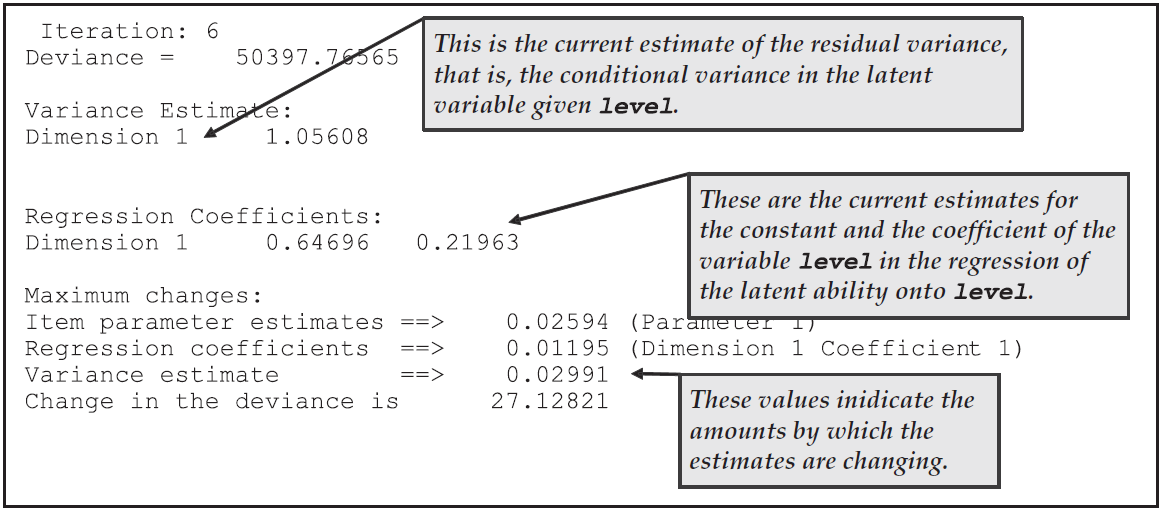
Figure 2.42: Reported Information on Estimation Progress for ex5a.cqc

Figure 2.43 shows the contents of the file ex5a_shw.txt. The values reported here are the parameter estimates for the population component of the ACER ConQuest model — in this case, a regression of the latent ability onto grade level. In these data, the level variable was coded as 0 for the lower grade and 1 for the upper grade, so the results shown in Figure 2.43 indicate that the estimated mean of the lower grade is 0.671 and the mean of the upper grade is 0.231 higher (mean of higher grade=0.902). The conditional variance in the latent variable is estimated to be 1.207. If an item response model is fitted without the regression variable, the estimated mean and variance of the latent ability are 0.80 and 1.219 respectively.¹⁸

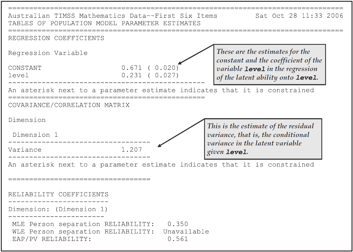
Figure 2.43: Population Model Parameter Estimates

The command file ex5a.cqc also produces the files ex5a_mle.txt and ex5a_eap.txt. These files contain latent ability estimates for each of the 6800 students in the file ex5_dat.txt. The format of these files is as follows. The file ex5a_mle.txt contains one line of data for each student in the sample who provided a valid response to at least one of the six items that we have analysed—in this sample, 6778 students. Columns 1 through 5 contain an identification number for the case, which is the sequence number of the student in the original data file. Columns 6 through 15 contain the total score that the student attained, columns 16 through 26 contain the maximum possible score that the student could have attained, columns 27 through 37 contain the maximum likelihood estimate of the student’s latent ability, and columns 38 through 48 provide an asymptotic standard error for that ability estimate. An extract from ex5a_mle.txt is shown in Figure 2.44.

EXTENSION: The maximum likelihood estimation method does not provide finite latent ability estimates for students who receive a score of zero or students who achieve the maximum possible score on each item. ACER ConQuest produces finite estimates for zero and maximum scorers by estimating the abilities that correspond to the scores r and M–r where M is the maximum possible score and r is an arbitrarily specified real number. In ACER ConQuest, the default value for r is 0.3. This value can be changed with the set command argument zero/perfect=r.

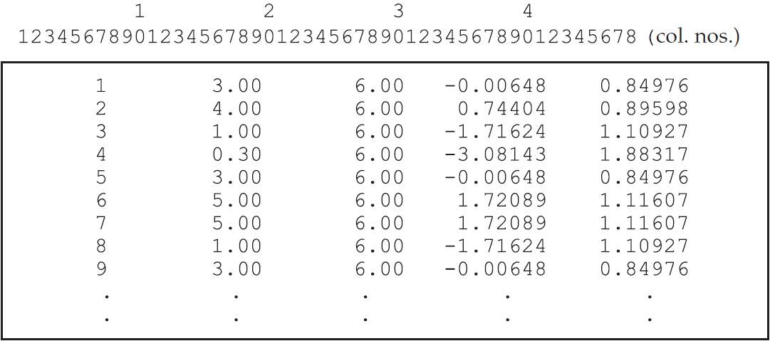
Figure 2.44: An Extract from the MLE File ex5a_mle.txt

The file ex5a_eap.txt contains three lines of data for each student in the sample who provided a valid response to at least one of the six items that we have analysed—in this case, 20 334 lines. The first line contains an identification number, which is the sequence number of the student in the original data file. The second line contains the expected value of the student’s posterior latent ability distribution—the so-called EAP ability estimate. The third line is the variance of the student’s posterior latent ability distribution; this can be used as the error variance for the EAP ability estimate. An extract from ex5a_eap.txt is shown in Figure 2.45.

WARNING: The maximum likelihood estimate is a function of the item response data only; as such, it is not influenced by the population model. The EAP estimates are a function of both the population model and the item response model, so a change in the population model will result in a change in the EAP estimates.

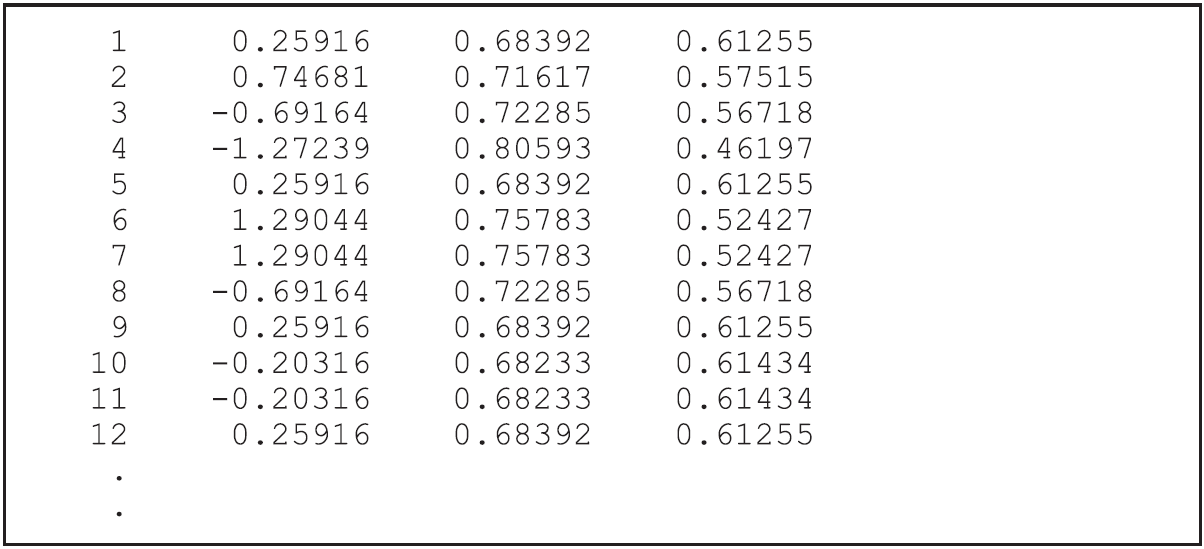
Figure 2.45: An Extract from the EAP File ex5a_eap.txt

2.6.1.4 Comparing Latent Regression with OLS Regression

If the file ex5a_mle.txt is merged with the level variable for each case, it is possible to regress the maximum likelihood ability estimates onto level. Similarly, if the file ex5a_eap.txt is merged with the level variable, a regression of EAP estimates onto level can be carried out. The results obtained from these two regression analyses can be compared (see Figure 2.43). For the purposes of this comparison, we have also fitted a model without any regressors and added the EAP ability estimates from this run to the file ex5a.out, which we have provided.¹⁹

The results of ordinary least squares (OLS) regressions of the various estimates of latent ability onto level are shown in Figure 2.46.

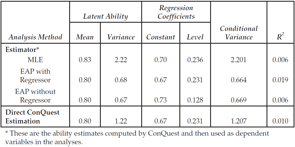
Figure 2.46: OLS Regression Results Using Alternative Latent Ability Estimates

The last row of the table contains the results produced directly by ACER ConQuest. Theoretical and simulation studies by Mislevy (Mislevy, 1984, 1985) and Adams, Wilson, & Wu (1997) indicate that the ACER ConQuest results are the ‘correct’ results. The results in the table show that the mean of the latent ability is reasonably well estimated from all three estimators. The slight overestimation that occurs when using the MLE estimator is likely due to the ad-hoc approach that must be applied to give finite ability estimates to those students with either zero or perfect scores. The variance is overestimated by the MLE estimator and underestimated by the two EAP estimators. The overestimation of variance from the MLE ability estimator results from the independent measurement error component (Wright & Stone, 1979) and a slight ‘outwards’ bias in the MLE estimates (Lord, 1983, 1984). The underestimation of variance from the EAP ability estimators results from the fact that the EAP estimates are ‘shrunken’ (Lord, 1983, 1984).

EXTENSION: In section 2.9, we will discuss plausible values, the use of which enables the unbiased estimation of the parameters of any submodel of the population model that is specified in the ACER ConQuest analysis and is used to generate the plausible values.

For the regression model, we note that MLE estimates are reasonably close to the ACER ConQuest results, the EAP estimates produced with the use of the regressor give results the same as those produced by ACER ConQuest, and the EAP estimates produced without the regressor overestimate the constant term and underestimate the level effect. As was the case with the means, the difference between the MLE-based estimates and the ACER ConQuest-based estimates for the constant term is likely due to the ad-hoc treatment of zero and perfect scores when ACER ConQuest generates the maximum likelihood point estimates. The EAP estimates produced with the use of the regressor give unbiased estimates of the regression coefficients, while the estimates produced with the EAP without regressor are shrunken. The conditional variances behave in the same fashion as the (unconditional) variance of the latent ability.

None of the point estimators of students’ latent abilities can be relied upon to produce unbiased results for all of the parameters that may be of interest. This is particularly true for short tests, as is the case here. When tests of 15 or more items are used, both MLE and EAP estimators will produce results similar to those produced directly by ACER ConQuest.

2.6.2 b) Avoiding the Problem of Measurement Error

The differences between the regression results that are obtained from ACER ConQuest and from the use of ordinary least squares using the various point estimates of latent ability can be avoided by using longer tests. In Section 2.6.2.2 below we present the command file ex5b.cqc, which reads and analyses all of the items in the file ex5_dat.txt.

2.6.2.1 Required files

The files that we use in this second sample analysis are:

filename	content
ex5b.cqc	The command statements used for the second analysis.
ex5_dat.txt	The data.
ex5_lab.txt	The variable labels for the items.
ex5b_prm.txt	Initial values for the item parameter estimates.
ex5b_reg.txt	Initial values for the regression parameter estimates.
ex5b_cov.txt	Initial values for the variance parameter estimates.
ex5b_shw.txt	Selected results of the analysis.
ex5b_eap.txt	Expected a-posterior ability estimates for the students.

(The last two files will be created when the command file is executed.)

2.6.2.2 Syntax

ex5b.cqc is the command file used in the second sample analysis for a Latent Variable t-Test (158 Items). The file is shown in the code box below. The list underneath the code box explains each line of commands.

ex5b.cqc:

datafile ex5_dat.txt;
title     Australian TIMSS Mathematics Data--All Items; 
format    gender 17 level 18 gbyl 19 responses 20-176;
labels  << ex5_lab.txt;
codes 0,1,2,3,4,5,M;
recode (R) (.);
key 
13442341153114122133113244235223341323324535
24322331211313511511324113143242223435112411
14141221331131232441221432233421354221332511
2253131111111111111111141!1;
key 
XXXXXXXXXXXXXXXXXXXXXXXXXXXXXXXXXXXXXXXXXXXX
XXXXXXX2X2XXXXX22XXXXXX2XX2XXXXXXXXXXXX2XXXX
XX2X2XX2XXXXX2XXXXX2XX2XXXXXXXX2XXXXXXXXXX2X
XXXXXX22222222222222222X2!2;
key 
XXXXXXXXXXXXXXXXXXXXXXXXXXXXXXXXXXXXXXXXXXXX
XXXXXXX3X3XXXXX33XXXXXX3XX3XXXXXXXXXXXX3XXXX
XX3X3XX3XXXXX3XXXXX3XX3XXXXXXXX3XXXXXXXXXX3X
XXXXXX33333333333333333X3!3;
regression level;
model item+item*step;
import init_parameters << ex5b_prm.txt;
import init_reg_coefficients << ex5b_reg.txt;
import init_covariance << ex5b_cov.txt;
estimate !fit=no,stderr=quick;
set p_nodes=1000;
show !table=3 >> Results/ex5b_shw.txt;
show cases !estimate=eap >> Results/ex5b_eap.txt;

Lines 1-4
As for ex5a.cqc (discussed in Section 2.6.1.2), except the title statement has been changed to indicate all items are being analysed rather than the first six and the response block in the format statement has been enlarged to include all 158 responses.
Line 5
In this analysis, we would like to treat the data coded R as missing-response data and the data coded M as incorrect. It is necessary therefore to make an explicit list of codes that excludes the R. This is in contrast to the previous sample analysis in which we did not provide a code list. In that case, all data in the file were regarded as legitimate, and those responses not matching a key were scored as incorrect.
Line 6
Here the R code is recoded to . (period), one of the default missing-response codes. Strictly speaking, this recode statement is unnecessary since the absence of the R in the code string will ensure that it is treated as missing-response data. It is added here as a reminder that R is being treated as missing-response data.
Lines 7-21
The key statement argument is now 158 characters long because there are 158 items. This test contains a mixture of multiple choice, short answer and extended response items, so we are using three key statements to deal with the fact that the short answer and extended response items are already scored. The first key argument contains the keys for the multiple choice items; and for short answer and extended response items, the code 1 has been entered. Any matches to this key argument will be recoded to 1, as shown by the option. In other words, correct answers to multiple choice items will be recoded to 1; and for the short answer and extended response items, 1 will remain as 1. All other codes will be recoded to 0 (incorrect) after the last key statement and any recode statements have been read. The second and third key statements contain the character X for the multiple choice items and 2 and 3 respectively for the short answer and extended response items. As X does not occur in the response block of the data file, these key statements will have no effect on the multiple choice items (correct answers to which have been recoded to 1 by the first key statement), but the short answer and extended response items will have code 2 scored as 2 and code 3 scored as 3. While the second and third key statements don’t change the codes, they prevent the 2 and 3 codes in the short answer and extended response items from being recoded to 0, as would have occurred if only one key statement were used.

EXTENSION: ACER ConQuest uses the Monte Carlo method to estimate the mean and variance of the marginal posterior distributions for each case. The system value p_nodes (The default is 2000, and this can be changed using the command set with the argument p_nodes) governs the number of random draws in the Monte Carlo approximations of the integrals that must be computed.

WARNING: For cases with extreme latent ability estimates, the variance of the marginal posterior distribution may not be estimated accurately if p_nodes is small. Increasing p_nodes will improve the variance estimates. On the other hand, for EAP estimates, moderate values of p_nodes are sufficient.
Line 22
As for line 6 of ex5a.cqc (see Section 2.6.1.2).
Line 23
This model statement yields the partial credit model. In the previous sample analysis, all of the items were dichotomous, so a model statement without the item*step term was used. Here we are specifying the partial credit model because it will deal with the mixture of dichotomous and polytomous items in this analysis.
Lines 24-26
This analysis takes a considerable amount of time, so initial value files are used to import a set of starting values for the item, regression and variance parameter estimates.
Line 27
In this sample analysis, we are not concerned with the properties of the items, so we are specifying the fit=no option to speed up the analysis.
Line 28
The set command is used to alter some of ACER ConQuest’s default values. The p_nodes=1000 argument requests that 1000 nodes be used when EAP estimates are produced and when plausible values are drawn. The default value for p_nodes is 2000. Reducing this to 1000 decreases the time necessary to compute EAP estimates.
Line 29
This show statement writes the population model parameter estimates (table 3) to ex5b_shw.txt.
Line 30
This show statement writes a file containing the EAP ability estimate for each case.

2.6.2.3 Running the Second t-Test Sample Analysis

To run this sample analysis, start the GUI version of ACER ConQuest and open the control file Ex5b.cqc.

Select Run\(\rightarrow\)Run All. ACER ConQuest will begin executing the statements that are in the file ex5b.cqc; and as they are executed, they will be echoed in the Output Window. When ACER ConQuest reaches the estimate statement, it will begin fitting the partial credit model to the data. In this case, only two iterations will be necessary because the initial values that were provided in the files ex5b_prm.txt, ex5b_reg.txt and ex5b_cov.txt are the output of a full analysis that have been performed on a previous occasion.

Figure 2.47 shows the contents of ex5b_shw.txt. A comparison of the results reported here with those reported in Figure 2.43 is quite interesting. Recall that the results in Figure 2.43 are from fitting a similar latent regression model to the first six items only — the set of items taken by all students. What we note is that the variance estimates are very similar, as is the regression coefficient for level. In fact, this similarity is quite remarkable given that the first analysis used only six of the 158 items and approximately one-fifth of the data that were actually available. The CONSTANT terms are quite different. The difference between the estimates for the CONSTANT is due to the model identification constraint. In the previous analysis, the item response model was identified by setting the mean difficulty of the first six items to zero. In this second run, the mean difficulty of all 158 items is set to zero.

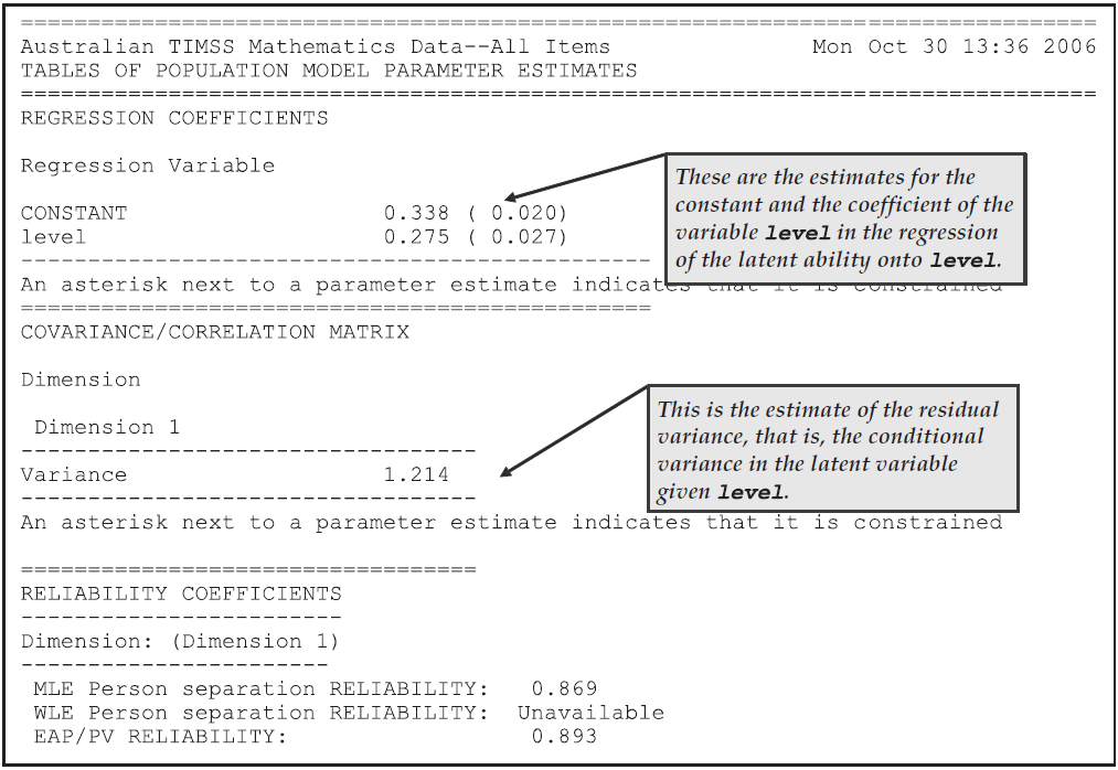
Figure 2.47: Population Model Parameter Estimates

2.6.2.4 Comparing Latent Regression with OLS Regression for the Second Sample Analysis

As with the previous sample analysis, we produced a file of EAP ability estimates and then merged these with the level variable for each case. For the purposes of this comparison, we have also fitted a model without any regressors and added the EAP ability estimates from this run to the file ex5b.out, which we have provided.²⁰ Figure 2.48 shows the results of regressing these EAP estimates onto level and compares the results obtained with those obtained by ACER ConQuest.

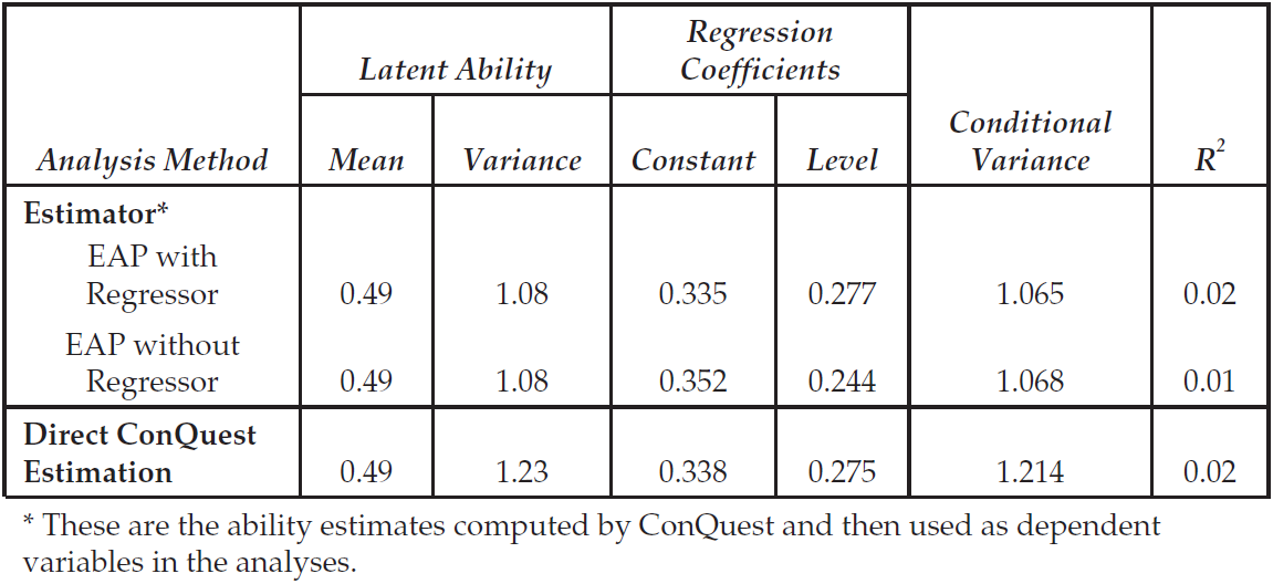
Figure 2.48: OLS Regression Results Using Alternative Latent Ability Estimates

The mean is well estimated by the EAP latent ability estimates, but as in the previous sample analysis the variance is underestimated. The degree of underestimation is much less marked than it was in the previous sample analysis, but it is still noticeable. For the regression coefficients, we note that the EAP with regressor latent ability estimates are very close to the values produced by ACER ConQuest. The EAP without regressor values are moderately biased, again due to their shrunken nature: the CONSTANT term is overestimated and the difference between the levels is underestimated. The conditional variances are again under-estimated by the EAP-based ability estimates.

2.6.3 c) Latent Multiple Regression

The regressions undertaken in the last two sample analyses used a single regressor, level, which takes two values, 0 to indicate lower grade and 1 to indicate upper grade. This effectively meant that these two sample analyses were equivalent to two-sample t-tests. In ACER ConQuest, up to 200 regression variables can be used simultaneously, and the regressors can be continuous numerical values. As a final sample analysis, we will show the results of analysing the data in ex5_dat.txt using three regressors.

2.6.3.1 Syntax

The command file for this sample analysis (ex5c.cqc) is given in the code box below. The only substantive difference between ex5b.cqc (cf. Section 2.6.2.2) and ex5c.cqc is in line 19, where the variables gender and gbyl are added.

ex5c.cqc:

datafile ex5_dat.txt;
title  Australian TIMSS Mathematics Data-All Items; 
format gender 17 level 18 gbyl 19 responses 20-176;
labels  << ex5_lab.txt;
codes 0,1,2,3,4,5,M;
recode (R) (.);
key 
1344234115311412213311324423522334132332453524322331211313511
5113241131432422234351124111414122133113123244122143223342135
42213325112253131111111111111111141!1;
key 
XXXXXXXXXXXXXXXXXXXXXXXXXXXXXXXXXXXXXXXXXXXXXXXXXXX2X2XXXXX22
XXXXXX2XX2XXXXXXXXXXXX2XXXXXX2X2XX2XXXXX2XXXXX2XX2XXXXXXXX2XX
XXXXXXXX2XXXXXXX22222222222222222X2!2;
key 
XXXXXXXXXXXXXXXXXXXXXXXXXXXXXXXXXXXXXXXXXXXXXXXXXXX3X3XXXXX33
XXXXXX3XX3XXXXXXXXXXXX3XXXXXX3X3XX3XXXXX3XXXXX3XX3XXXXXXXX3XX
XXXXXXXX3XXXXXXX33333333333333333X3!3;
regression level gender gbyl;
model item+item*step;
import init_parameters << ex5c_prm.txt;
import init_reg_coefficients << ex5c_reg.txt;
import init_covariance << ex5c_cov.txt;
estimate !fit=no,stderr=quick;
show !table=3 >> Results/ex5c_shw.txt;
set p_nodes=1000;
show cases !estimate=eap >> Results/ex5c_eap.txt;

NOTE: The ACER ConQuest population model is a regression model that assumes normality of the underlying latent variable, conditional upon the values of the regression variables. If you want to regress latent ability onto categorical variables or to specify interactions between variables, then appropriate contrasts and interaction terms must be created external to the ACER ConQuest program. For instance, in this sample analysis, we have constructed the interaction between gender and level by constructing the new variable gbyl, which is the product of gender and level, and adding it to the data file.

2.6.3.2 Running the Latent Multiple Regression Analysis

Figure 2.49 shows the contents of ex5c_shw.txt, the population model parameter estimates for this third latent multiple regression sample analysis. The results reported in the figure show that the main effects of grade (level) and gender are 0.251 and –0.030, respectively, while the interaction between gender and grade (gbyl) is 0.052. The CONSTANT (0.351) is the estimated mean for male students in the lower grade. The estimated mean of female students in the lower grade is 0.321 (=0.351–0.030), of male students in the upper grade is 0.602 (=0.351+0.251), and of female students in the upper grade is 0.624 (=0.351+0.251 – 0.030+0.052).

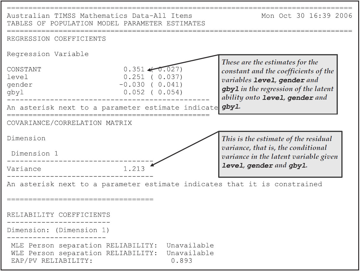
Figure 2.49: Population Model Parameter Estimates for the Latent Multiple Regression Sample Analysis

2.6.4 Summary

In this section, we have seen how to use ACER ConQuest to fit unidimensional latent regression models. Our sample analyses have been concerned with using categorical regressors, but ACER ConQuest can analyse up to 200 continuous or categorical regressors. Some key points covered in this section are:

Secondary analyses using EAP and MLE ability estimates do not produce results that are equivalent to the ‘correct’ latent regression results. The errors that can be made in a secondary analysis of latent ability estimates are greater when measurement error is large.
The key command can be used with a mixture of dichotomous and polytomous items.
The show command can be used to create files of ability estimates. ACER ConQuest provides both EAP and maximum likelihood ability estimates.
The import command can be used to read files of initial values for parameter estimates.

2.7 Differential Item Functioning

Within the context of Rasch modelling an item is deemed to exhibit differential item functioning (DIF) if the response probabilities for that item cannot be fully explained by the ability of the student and a fixed set of difficulty parameters for that item. Through the use of its multi-faceted modelling capabilities, and more particularly its ability to model interactions between facets, ACER ConQuest provides a powerful set of tools for examining DIF.

In this section three examples are considered. In the first, ACER ConQuest is used to explore the existence of DIF with respect to gender in a short multiple-choice test. This is a traditional DIF analysis because it is applied to dichotomously scored items and examines DIF between two groups—that is, it uses a binary grouping variable. In the second example DIF is explored when the grouping variable is polytomous—in fact the grouping variable defines eight groups of students. Finally, in the third example DIF in some partial credit items is examined.

2.7.1 a) Examining Gender Differences in a Multiple Choice Test

2.7.1.1 Required files

The data used in this first example are the TIMSS data that were described in the previous section (2.6).

The files used in this example are:

filename	content
ex6a.cqc	The command lines used for the first analysis.
ex5_dat.txt	The data.
ex6_lab.txt	A file of labels for the items.
ex6a_shw.txt	Selected results from the analysis.

2.7.1.2 Syntax

The control code for analysing these data is contained in ex6a.cqc, as shown in the code box below. Each line of commands is explained in the list that follows the code.

ex6a.cqc:

datafile ex5_dat.txt;
title TIMSS Mathematics--First Six Items--Gender Differences;
format book 16 gender 17 level 18 gbyl 19 responses 20-25;
labels << ex6_lab.txt;
key 134423 ! 1;
model item-gender+item*gender;
estimate !fit=no,stderr=empirical;
show !table=2>> Results/ex6a_shw.txt;
plot icc! gins=1:2,overlay=yes,legend=yes;
plot icc! gins=3:4,overlay=yes,legend=yes;
plot icc! gins=5:6,overlay=yes,legend=yes;
plot icc! gins=7:8,overlay=yes,legend=yes;
plot icc! gins=9:10,overlay=yes,legend=yes;
plot icc! gins=11:12,overlay=yes,legend=yes;

Line 1
The data in ex5_dat.txt is to be used.
Line 2
Sets the title.
Line 3
Note that in this format we are reading the explicit variables book, gender, level and the product of gender and level from columns 16, 17, 18 and 19 respectively.
Line 4
Note that the labels file for this analysis contains labels for book, gender and item.
Line 5
Gives the scoring key.
Line 6
The model statement has three terms. These three terms involve two facets, item and gender. So, as ACER ConQuest passes over the data, it will identify all possible combinations of the item and gender variables and construct 12 (six items by 2 genders) generalised items. The model statement requests that ACER ConQuest describes the probability of correct responses to these generalised items using an item main effect, a gender main effect and an interaction between item and gender.

The first term will yield a set of item difficulty estimates, the second term will give the mean ability of the male and female students and the third term will give an estimate of the difference in the difficulty of the items for the two gender groups. Note, a negative sign (-) has been used in front of the gender term. This ensures that the gender parameters will have the more natural orientation of a higher number corresponding to a higher mean ability.
Line 7
Two options have been included with the estimate command. fit=no, means that fit statistics will not be computed, and stderr=empirical means that the more time consuming (and more accurate) method will be used to calculate asymptotic standard error estimates for the items. The more accurate method has been chosen for this analysis since the comparison of estimates of some parameters to their standard errors is used in judging whether there is DIF.
Line 8
The show command will write table 2 to the file ex6a_shw.txt.
Lines 9-14
Plots the item characteristic curves for each of the six items. Because this run of ACER ConQuest uses a multi-faceted model that involves six items and two genders there are actually 12 generalised items that are analysed. In the model statement the item facet is mentioned first and the gender facet is mentioned second, as a consequence the gender facet reference cycles fastest in the referencing of generalised items. That is, generalised item one corresponds to item one and gender one; generalised item two corresponds to item one and gender two; generalised item three corresponds to item two and gender one; generalised item four corresponds to item two and gender two; and so on.

Each plot command plots the item characteristic curves for two generalised items. For example the first command plots generalised items one and two, which corresponds to a plot of item one for the two gender groups separately. The overlay=yes option results in both item characteristic curves being plotted in the same graph.

2.7.1.3 Running the Test for DIF

To run this sample analysis, start the GUI version of ACER ConQuest and open the control file Ex6a.cqc.

Select Run\(\rightarrow\)Run All. ACER ConQuest will begin executing the statements that are in the file ex6a.cqc; and as they are executed they will be echoed in the Output Window. When it reaches the estimation command ACER ConQuest will begin fitting a multi-faceted model to the dichotomous data. TThe item parameter estimates will be written to the file ex6a_shw.txt.

The contents of ex6a_shw.txt are shown in Figure 2.50. The figure contains three tables, one for each of the terms in the model statement.

The first table shows the item difficulty parameter estimates for each of the six items.

The second table shows the estimates for the gender differences in ability estimates. A negative sign (-) was used for the gender term in the item response model so these results indicate that the male students have performed more poorly than the female students. The actual parameter estimate for the male students is three times larger than its standard error estimate so the difference between the male and female means is obviously significant. The chi-square value of 9.63 on one degree of freedom is consistent with this finding. The conclusion that can be drawn here is that the male mean performance is lower than that of the females, this DOES NOT indicate differential item functioning. Further, the estimated difference of 0.114 is small at just over 10% of a student standard deviation.²¹

The third table gives the interaction between the item and gender facets. The estimate of 0.060 for item BSMMA01 and males indicates that 0.060 must be added to the difficulty of this item for male students, similarly –0.060 must be added for the females. That is, female students found this item to be relatively easier than did the males. The results in this table show that three items (BSMMA03, BSMMA05 and BSMMA06) are relatively easier for males than females, two items (BSMMA01 and BSMMA04) are relatively easier for females than males, and one item (BSMMA02) has the same difficulty. The significant chi-square (155.00, df=5) also shows the existence of DIF.

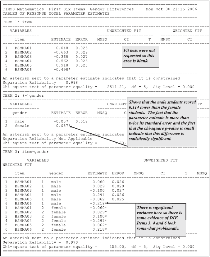
Figure 2.50: Parameter Estimates for DIF Examination in a Multiple Choice Test

NOTE: By including the main effect, gender, in the item response model, estimates of the mean scores for male and female students has been obtained. An alternative approach that would have achieved an identical result would have been to place the gender variable in the population model. It would not be appropriate to include gender in both the item response and the population models since this would make the model unidentified.

WARNING: The current version of ACER ConQuest assumes independence between the parameter estimates when computing the chi-square test of parameter equality.

While this analysis has shown the existence of DIF in these items it is the magnitude of that DIF that will determine if the effect of that DIF is of substantive importance. For example, the first item (BSMMA01) is significantly more difficult for males than females but the difference estimate is just 0.12 logits. If all of the items exhibited DIF of this magnitude it would shift the male ability distribution by just over 10% of a student standard deviation. With just one item having this DIF, the effect is much smaller. The fourth item (BSMMA04) exhibits much more DIF. In fact if all of the items in the test had behaved like this item the estimated mean score for the males would be 0.582 logits lower than that of the females, that is more than 50% of a student standard deviation.

Figure 2.51 shows the item characteristic curves for Item 4 for males and females separately. The dark (blue) curves are for males, and the light (green) curves are for females. It can be seen that, given a particular ability level, the probability of being successful on this item is higher for females than for males, i.e., females find this item easier than males.

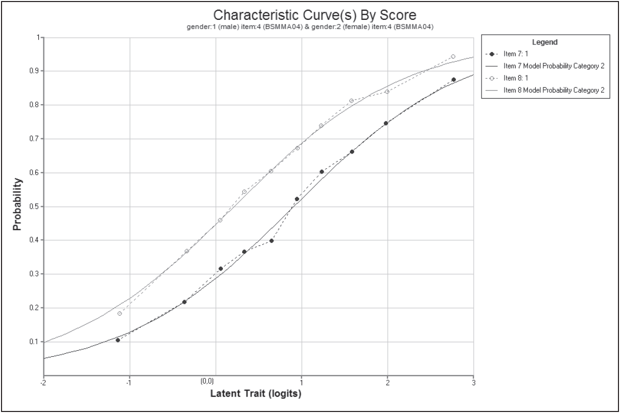
Figure 2.51: Item Characteristic Curves for Generalised Items Seven and Eight (Item 4, Males and Females)

2.7.2 b) Examining DIF When the Grouping Variable Is Polytomous

ACER ConQuest can also be used to examine DIF when the grouping variable is polytomous, rather than dichotomous, as is the case with gender.

2.7.2.1 Required files

In the TIMSS design the test items were allocated to eight different testing booklets and students were allocated one of the eight booklets at random. One way of testing whether the rotation scheme was implemented successfully is to estimate the mean ability estimates for the students who were assigned each booklet and to see if there is any evidence of DIF across the booklets.

The files that we will use in this example are:

filename	content
ex6b.cqc	The command lines used for the second analysis.
ex5_dat.txt	The data.
ex6_lab.txt	A file of labels for the items.
ex6b_shw.txt	Selected results from the analysis.

2.7.2.2 Syntax

The contents of the control file, ex6b.cqc, used in this analysis to examine booklet effect in a MC test, is shown in the code box below. The only command that is different here to ex6a.cqc (see Section 2.7.1.2) is the model statement, in which the variable book rather than gender is used.

ex6b.cqc:

datafile ex5_dat.txt;
title Australian TIMSS Mathematics Data--First Six Items--Booklet Differences; 
format  book 16 gender 17 level 18 gbyl 19 responses 20-25;
labels  << ex6_lab.txt;
key  134423 ! 1;
model item+book+item*book;
estimate !fit=no;
show !table=2 >> Results/ex6b_shw.txt;

2.7.2.3 Running the Test for DIF when the Grouping Variable is Polytomous

After running this analysis using the same procedures as described for previous examples, the file ex6b_shw.txt will be produced, the contents of which are shown in Figure 2.52.

This figure shows that there is no statistically significant book effect and that there is no between booklet DIF.

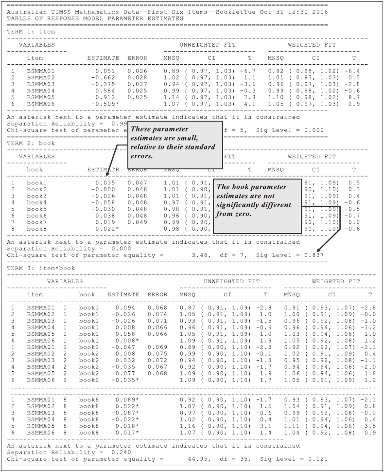
Figure 2.52: Parameter Estimates for DIF Examination Across Booklets

2.7.3 c) DIF for Polytomous Items

As a final example on DIF, a set of polytomous items is examined.

2.7.3.1 Required files

The data were collected by Adams et al. (1991) as a part of their study of science achievement. The set of items that are analysed formed an instrument that assessed students’ understanding of force and motion.

The files used in this example are:

filename	content
ex6c.cqc	The command lines used for the third set of analyses.
ex6_dat.txt	The data.
ex6c_lab.txt	The variable labels for the items on the test.
ex6c_shw.txt	The results of an analysis that includes gender by step interactions.
ex6d_shw.txt	The results from an analysis that does not include gender by step interactions.

2.7.3.2 Syntax

The control code for this example (ex6c.cqc) is shown in the code box below. ex6c.cqc is very similar to the command files of earlier examples in this section (ex6a.cqc and ex6b.cqc), so only the distinguishing aspects of ex6c.cqc are commented upon in the list underneath the code box.

Note that in this case the control code will actually run two ACER ConQuest analyses.

ex6c.cqc:

datafile ex6_dat.txt;
format responses 10-18 grade 118 gender 119!tasks(9);
set warnings=no;
model tasks - gender + tasks*gender + gender*tasks*step;
labels << ex6c_lab.txt;
estimate;
show!table=1:2 >> Results/ex6c_shw.txt;
plot expected! gins=1:2,overlay=yes,legend=yes;
reset;

datafile ex6_dat.txt;
format responses 10-18 grade 118 gender 119!tasks(9);
set warnings=no;
model tasks-gender+tasks*gender+tasks*step;
labels << ex6c_lab.txt;
estimate!fit=no,stderr=empirical;
show!table=1:2 >> Results/ex6d_shw.txt;
plot expected! gins=1:2,overlay=yes,legend=yes;

Line 4
This model includes four terms. Two main effects, tasks and gender, give the difficulty of each of the tasks and the means of the two gender groups. The interaction tasks*gender models the variation in difficulty of the task between the two genders and finally the gender*tasks*step term models differing step structures for each task and gender.

EXTENSION: In this example randomly chosen students from both an upper and lower grade responded to all of the tasks so the use of grade as a regressor is not necessary to produce consistent estimates of the item response model parameters.

If the sub-samples of students who respond to specific test tasks were systematically different in their latent ability distribution then the use of a regressor will be necessary to produce consistent parameter estimates for the item response model (Mislevy & Sheehan, 1989).
Line 9
The reset command separates sets of analyses to be run.
Line 14
This model command is similar to the previous one in that it has four terms. The difference is that the final term does not include variation between males and females in the task’s step structure. Comparing the fit of this model to the model given by line 4, we can assess the need for a step structure that is different for male and female students.

2.7.3.3 Running the Analysis

After this analysis is run using the same procedures as described for previous examples, the files ex6c_shw.txt and ex6d_shw.txt will be produced. An extract of ex6c_shw.txt is given in Figure 2.53, it shows that there is no difference between the overall performance of male and female students and that there is no interaction between gender and task difficulty. In this figure the parameter estimates for the term gender*tasks*step are not shown because the easiest way to test whether the step structure is the same for the male and female students is to compare the deviance of the two models that were fitted by the code in ex6c.cqc.

The results reported in Figure 2.53 show that the model with a step structure that is invariant to gender does not fit as well as the model with a step structure that varies with gender. The conclusion that can be drawn from these analyses is that while the overall male and female performance is equivalent, as are the difficulty parameters for each of the tasks it appears that male and female students have differing step structures. A closer examination of the difference in the step structures between male and female students would appear to be required.

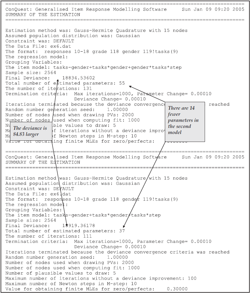
Figure 2.53: The Summary Tables for the Two Polytomous DIF Analyses

To illustrate the differences between these two models, the expected score curves have been plotted for the first two generalised items for each model. The plots are shown in Figure 2.54. The first plot shows the expected score curves when a different step structure is used for male and female students, while the second plot shows the expected score curves when a common step structure is used. In the second plots the curves are parallel, in the sense that they have the same shape but are just displaced on the horizontal axes. In the first plots the expected curves take a different shape, and in fact cross.

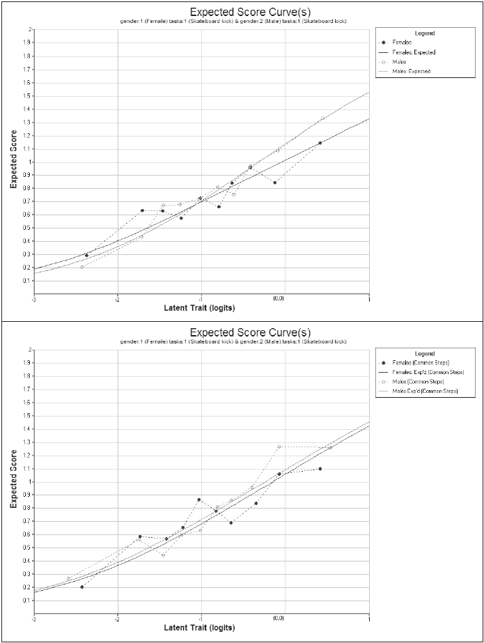
Figure 2.54: Output from Analysis of DIF in Polytomous Items

2.7.4 Summary

In this section we have illustrated how ACER ConQuest can be used to examine DIF with dichotomous items and polytomous items, and how DIF can be explored where the grouping variable is polytomous.

Some key points covered in this section are:

Modelling DIF can be done through adding an item-by-facet interaction term in the model statement.
Item characteristic curves can be plotted with the overlay option.
A comparison of model fit can be carried out using the deviance statistic.
Expected score curves are useful for polytomous items.
Different steps structures can be specified using the model statement.

2.8 Multidimensional Models

ACER ConQuest analyses are not restricted to models that involve a single latent dimension. ACER ConQuest can be used for the analysis of sets of items that are designed to produce measures on up to 30 latent dimensions.²² In this section, multidimensional models are fitted to data that were analysed in previous sections using a one-dimensional model. In doing so, we are able to use ACER ConQuest to explicitly test the unidimensionality assumption made in the previous analyses. We are also able to illustrate the difference between derived estimates and ACER ConQuest’s direct estimates of the correlation between latent variables. In this section, we also introduce the two different approaches to estimation (quadrature and Monte Carlo) that ACER ConQuest offers; and in the latter part of the section, we discuss and illustrate two types of multidimensional tests: multidimensional between-item and multidimensional within-item tests.

2.8.1 Example A: Fitting a Two-Dimensional Model

In the first sample analysis in this section, the data used in section 2.2 is re-analysed. In that section, we described a data set that contained the responses of 1000 students to 12 multiple choice items, and the data were analysed as if they were from a unidimensional set of items. This was a bold assumption, because these data are actually the responses of 1000 students to six mathematics multiple choice items and six science multiple choice items.

2.8.1.1 Required files

The files used in this sample analysis are:

filename	content
ex7a.cqc	The command statements.
ex1_dat.txt	The data.
ex1_lab.txt	The variable labels for the items on the multiple choice test.
ex7a_shw.txt	The results of the Rasch analysis.
ex7a_itn.txt	The results of the traditional item analyses.
ex7a_eap.txt	The EAP ability estimates for the students.
ex7a_mle.txt	The maximum likelihood ability estimates for the students.

2.8.1.2 Syntax

The contents of the command file ex7a.cqc are shown in the code box below, and explained line-by-line in the list that follows the figure.

ex7a.cqc:

datafile ex1_dat.txt;
format id 1-5  responses 12-23;
labels << ex1_lab.txt;
key acddbcebbacc ! 1;
score (0,1) (0,1) ()! items(1-6);
score (0,1) () (0,1)! items(7-12);
model item;
estimate ;
show !estimates=latent,tables=1:2:3:9>> Results/ex7a_shw.txt;
itanal >> Results/ex7a_itn.txt;
show cases !estimates=eap >> Results/ex7a_eap.txt;
show cases !estimates=mle >> Results/ex7a_mle.txt;

Line 1
Indicates the name and location of the data file. Any name that is valid for the computer you are using can be used here.
Line 2
The format statement describes the layout of the data in the file ex1_dat.txt.
Line 3
Reads a set of item labels from the file ex1_lab.txt.
Line 4
Recodes the correct responses to 1 and all other values to 0.
Lines 5-6
The fact that a multidimensional model is to be fitted is indicated by the score statement syntax. In our previous uses of the score statement, the argument has had two lists, each in parentheses—a from list and a to list. The effect of those score statements was to assign the scores in the to list to the matching codes in the from list. If a multidimensional model is required, additional to lists are added. The arguments of the two score statements here each contain three lists. The first is the from list and the next two are to lists, one for each of two dimensions. The first six items are scored on dimension one; hence, the second to list in the first score statement is empty. The second six items are scored on the second dimension; hence, the first to list in the second score statement is empty.
Line 7
The simple logistic model is used.
Line 8
The model will be estimated using default settings.

NOTE: The default settings will result in a Gauss-Hermite method that uses 15 nodes for each latent dimension when performing the integrations that are necessary in the estimation algorithm. For a two-dimensional model, this means a total of 15 × 15 = 225 nodes. The total number of nodes that will be used increases exponentially with the number of dimensions, and the amount of time taken per iteration increases linearly with the number of nodes. In practice, we have found that 5000 nodes is a reasonable upper limit on the total number of nodes that can be used.
Line 9
This show statement writes tables 1, 2, 3, and 4 into the file ex7a_shw.txt. Displays of the ability distribution will represent the distribution of the latent variable.
Line 10
The itanal statement writes item statistics to the file ex7a_itn.txt.
Line 11
This show statement writes a file containing EAP ability estimates for the students on both estimated dimensions.
Line 12
This show statement writes a file containing maximum likelihood ability estimates for the students on both estimated dimensions.

2.8.1.3 Running the Two-Dimensional Sample Analysis

To run this sample analysis, start the GUI version of ACER ConQuest and open the control file Ex7a.cqc.

Select Run\(\rightarrow\)Run All. ACER ConQuest will begin executing the statements that are in the file ex7a.cqc; and as they are executed, they will be echoed in the Output Window. When ACER ConQuest reaches the estimate statement, it will begin fitting a multidimensional form of Rasch’s simple logistic model to the data. As it does so, it will report on the progress of the estimation.

Figure 2.55 is a sample of the information that will be reported by ACER ConQuest as it iterates to find the parameter estimates.

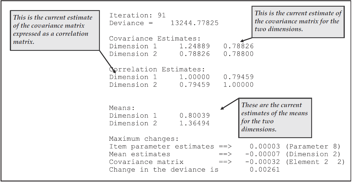
Figure 2.55: Reported Information on Estimation Progress for ex7a.cqc

In Figure 2.56, we have reported the first table (table 1) from the file ex7a_shw.txt. From this figure, we note that the multidimensional model has estimated 15 parameters; they are made up of 10 item difficulty parameters, the means of the two latent dimensions, and the three unique elements of the variance-covariance matrix. Ten item parameters are used to describe the 12 items because identification constraints are applied to the last item on each dimension.

The deviance for this model is 13244.73. If we refer back to Figure 2.9, we note that a unidimensional model when fitted to these data required the estimation of 13 parameters — 11 item difficulty parameters, one mean, and one variance — and the deviance was 13274.88. As the unidimensional model is a submodel of the two-dimensional model, the difference between the deviance of these two models is distributed as a chi-square with two degrees of freedom. Given the estimated difference of 30.1 in the deviance, we conclude that the unidimensional model does not fit these data as well as the two-dimensional model does.

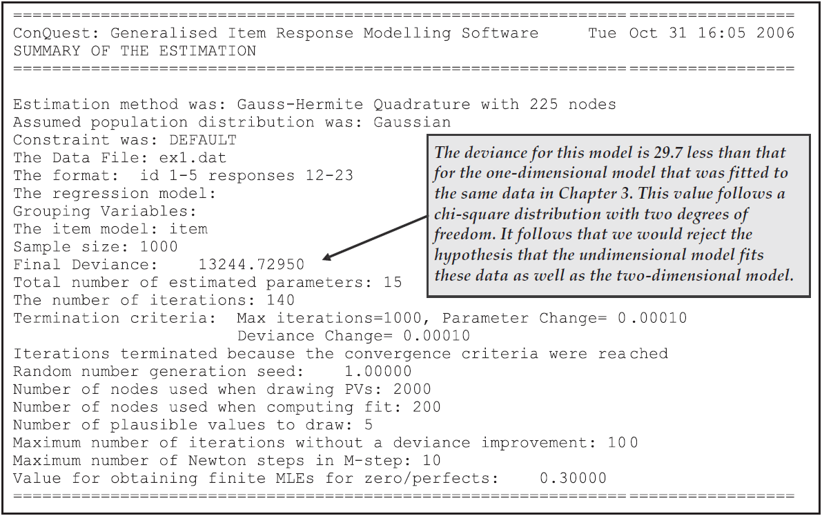
Figure 2.56: Summary Information for the Two-Dimensional Model

Figure 2.57 shows the second table (table 2) that is produced by the first show statement. It contains the item difficulty estimates and the fit statistics. It is interesting to note that the fit statistics reported here are almost identical to those reported for the unidimensional model. Note also that two of the item parameters are constrained. For identification purposes, the mean of the item parameters on each dimension is constrained to be zero. This is achieved by choosing the difficulty of the last item on each dimension to be equal to the negative sum of the difficulties of the other items on the dimension. As an alternative approach, it is possible to use the lconstraints argument of the set command to force the means of the latent variables to be set at zero and to allow all item parameters to be free.

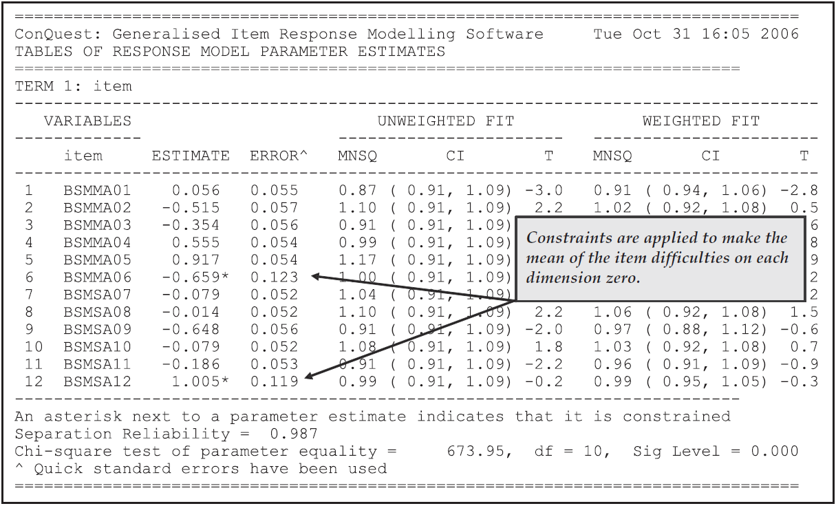
Figure 2.57: Item Parameter Estimates for the Two-Dimensional Model

Figure 2.58 shows the estimates of the population parameters as they appear in the third table (table 3) in file ex7a_shw.txt.

The first panel of the table shows that the estimated mathematics mean is 0.800 and the estimated science mean is 1.363.

NOTE: This does not mean that this sample of students is more able in science than in mathematics. The origin of the two scales has been set by making the mean of the item difficulty parameters on each dimension zero, and no constraints have been placed upon the variances. Thus, these are two separate dimensions; they do not have a common unit or origin.

The second panel of the table shows the variances, covariance and correlation for these two dimensions. The correlation between the mathematics and science latent variables is 0.774. Note that this correlation is effectively corrected for any attenuation caused by measurement error.

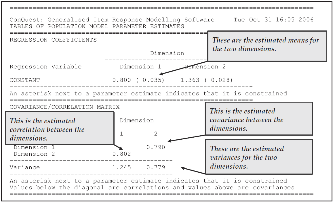
Figure 2.58: Population Parameter Estimates for the Two-Dimensional Model

Figure 2.59 is the last table (table 4) from the file ex7a_shw.txt. The left panel shows a representation of the latent mathematics ability distribution, and the right panel indicates the difficulty of the mathematics items. In the unidimensional equivalent of this figure, the items are plotted so that a student with a latent ability estimate that corresponded to the level at which the item was plotted would have a 50% chance of success on that item. For the multidimensional case, each item is assigned to a single dimension. A student whose latent ability estimate on that dimension is equal to the difficulty estimate for the item would have a 50% chance of success on that item.

EXTENSION: If quadrature-based estimation is used, the computation time needed to fit multidimensional models increases rapidly as additional dimensions are added. This can be alleviated somewhat by reducing the number of nodes being used, although reducing the number of nodes by too much will affect the accuracy of the parameter estimates. With this particular sample analysis, the use of 10 nodes per dimension results in variance estimates that are greater than those obtained using 20 nodes per dimension and the deviance is somewhat higher. If 30 nodes per dimension are used, the results are equivalent to those obtained with 20 nodes.

If you want to explore the possibility of using quadrature with less than 20 nodes per dimension, then we recommend fitting the model with a smaller number of nodes (e.g., 10) and then gradually increasing the number of nodes, noting the impact that the increased number of nodes has on parameter estimates, most importantly the variance. When you reach a point where increasing the number of nodes does not change the parameter estimates, including the variance, then you can have some confidence that an appropriate number of nodes has been chosen.

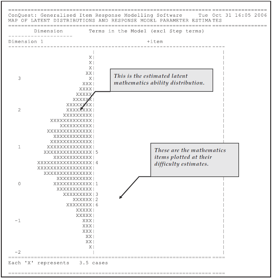
Figure 2.59: Map of the Latent Variables for the Two-Dimensional Model

2.8.1.4 Comparing the Latent Correlation with Other Correlation Estimates

The last two show statements in ex7a.cqc (see Section 2.8.1.2) produced files of students’ EAP and maximum likelihood ability estimates respectively. From these files we are able to compute the product moment correlations between the various ability estimates. In a run not reported here, we also fitted separate unidimensional models to the mathematics and science items and from those analyses produced EAP ability estimates. The various correlations that can be computed between mathematics and science are reported in Figure 2.60.²³

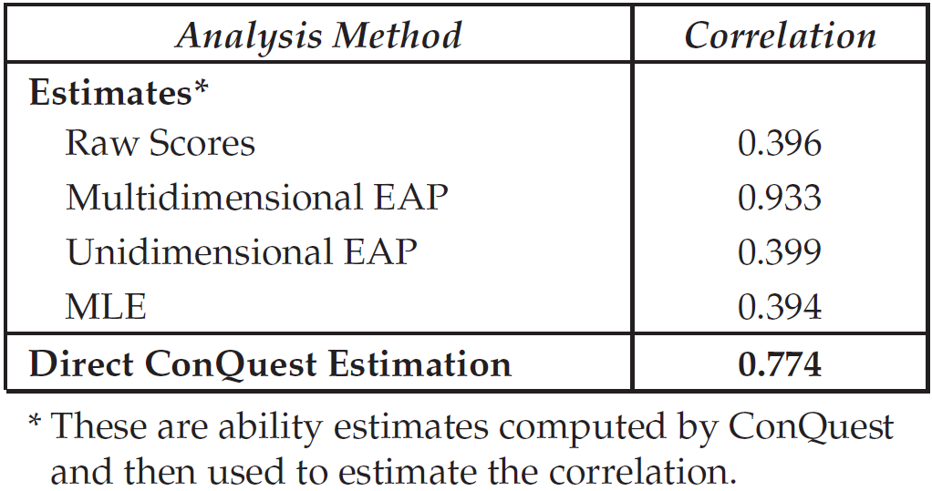
Figure 2.60: Comparison of Some Correlation Estimates with the Latent Ability Estimates

The estimates based on the raw score, unidimensional EAP, and MLE, which are all similar, indicate a correlation of about 0.40 between mathematics and science. All three estimates are attenuated substantially by measurement error. As the estimated KR-20 reliability of each of these dimensions is 0.58 and 0.43 respectively, an application of the standard ‘correction for attenuation’ formula yields estimated correlations of about 0.80.²⁴ This value is in fairly close agreement with the ACER ConQuest estimate. The correlation of 0.933 between the EAP estimates derived from the two-dimensional analysis is a dramatic overestimation of the correlation between these two variables and should not be used. This overestimation occurs because the EAP estimates are ‘shrunken’ towards each other. The degree of shrinkage is a function of the reliability of measurement on the individual dimensions; so if many items are used for each dimension, then all of the above indices will be in agreement.

EXTENSION: It is possible to recover the ACER ConQuest estimate of the latent ability correlation from the output of a multidimensional analysis by using plausible values instead of EAP estimates. Plausible values can be produced through the use of the cases argument and the estimates=latent option of the show command. Plausible values are discussed in section 2.9.

2.8.2 Example B: Higher-Dimensional Item Response Models

ACER ConQuest can be used to fit models of up to 15 or more dimensions, and we have routinely used it with up to eight dimensions. When analysing data with three or more dimensions, a Monte Carlo approach to the calculation of the integrals should be used.

2.8.2.1 Required files

In this sample analysis, we fit a five-dimensional model to some performance assessment data that were collected in Australia as part of the TIMSS study (Lokan et al., 1996). The data consist of the responses of 583 students to 28 items that belong to five different performance assessment tasks. These data are quite sparse because each student was only required to undertake a small subset of the tasks, but every task appears at least once with every other task.

The files that will be used in this sample analysis are:

filename	content
ex7b.cqc	The command statements.
ex7b.dat.txt	The data.
ex7b.lab.txt	The variable labels for the items.
ex7b.prm.txt	The estimates of the item response model parameters.
ex7b.reg.txt	The estimates of the regression coefficients for the population model.
ex7b.cov.txt	The estimates of the variance-covariance matrix for the population model.
ex7b.shw.txt	The results of the Rasch analysis.

2.8.2.2 Syntax

The command file ex7b.cqc is used in this Tutorial to fit a Higher-Dimensional Item Response Model. It is shown in the code box below, and each line of syntax is detailed in the list below the code.

ex7b.cqc:

title Australian Performance Assessment Data;
datafile ex7b.dat.txt;
format responses 1-28;
codes 0,1,2,3;
labels << ex7b.lab.txt;
recode (2) (1) !items(9,10);
recode (3) (2) !items(25);
score (0,1,2,3) (0,1,2,3) ( ) ( ) ( ) ( ) ! items (1-6);
score (0,1,2,3) ( ) (0,1,2,3) ( ) ( ) ( ) ! items (7-13);
score (0,1,2,3) ( ) ( ) (0,1,2,3) ( ) ( ) ! items (14-17);
score (0,1,2,3) ( ) ( ) ( ) (0,1,2,3) ( ) ! items (18-25);
score (0,1,2,3) ( ) ( ) ( ) ( ) (0,1,2,3) ! items (26-28);
model item+item*step;
export parameters >> ex7b.prm;
export reg_coefficients >>ex7b.reg;
export covariance >> ex7b.cov;
import init_parameters << ex7b.prm.txt;
import init_reg_coefficients <<ex7b.reg.txt;
import init_covariance << ex7b.cov.txt;
estimate ! method = montecarlo, nodes = 2000, conv = .005, stderr = quick;
show ! tables=1:2:3:4:9, estimates = latent >> Results/ex7b.shw.txt;

Line 1
Gives the title.
Line 2
Gives the name of the data file to be analysed. In this case, the data are contained in the file ex7b.dat.txt.
Line 3
The format statement indicates that there are 28 items, and they are in the first 28 columns of the data file.
Line 4
Restricts the valid codes to 0, 1, 2 or 3.
Line 5
A set of labels for the items are to be read from the file ex7b.lab.txt.
Lines 6-7
If a gap occurs in the scores in the response data for an item, then the next higher score for that item must be recoded downwards to close the gap. For example, in this data set, by coincidence, no response to item 9 or item 10 was scored as 1; all responses to these two items were scored as 0 or 2. To fill the gap between 0 and 2, the 2 has been recoded to 1 by the first recode statement. Similarly, for item 25, none of the response data is equal to 2, so 3 must be recoded to 2 to fill the gap.

NOTE: The model being fitted here is a partial credit model. Therefore, all score categories between the highest category and the lowest category must contain data. If this is not the case, then some parameters will not be identified. If warnings is not set to no, then ACER ConQuest will flag those parameters that are not identified and will indicate that recoding of the data is necessary. If warnings is set to no, then the parameters that are not identified due to null categories will not be reported. If a rating scale model were being fitted to these data, then recoding would not be necessary because all of the step parameters would be identified.
Lines 8-12
The model that we are fitting here is five dimensional, so the score statements contain six sets of parentheses as their arguments, one for the from codes and five for the to codes. The option of the first score statement gives the items to be assigned to the first dimension, the option of the second score statement gives the items to be allocated to the second dimension, and so on.
Line 13
The model we are using is the partial credit model.
Line 14
We want to update the export files of parameter estimates (see lines 15 through 17) every iteration, without warnings.
Lines 15-17
Request that item, regression and covariance parameter estimates be written to the files ex7b.prm.txt, ex7b.reg.txt, and ex7b.cov.txt respectively.
Lines 18-20
Initial values of item, regression and covariance parameter estimates are to be read from the files ex7b.prm.txt, ex7b.reg.txt, and ex7b.cov.txt respectively.
Line 21
This estimate statement has three arguments: method=montecarlo requests that the integrals that are computed in the estimation be approximated using Monte Carlo methods; nodes=2000 requests 2000 nodes be used in computing integrals; and converge=.005 requests that the estimation be terminated when the largest change in any parameter estimate between successive iterations becomes less than 0.005.

EXTENSION: Wilson & Masters (1993) discuss a method of dealing with data that have ‘null’ categories of the type we observe in these data for items 9, 10 and 25. Their approach can be implemented easily in ACER ConQuest by using a score statement that assigns a score of 2 to the category 1 of items 9 and 10 and a score of 3 to the category 2 of item 25, after recoding has been done to close the gaps.

NOTE: We have used the same names for the initial value and export files. These files must already exist so that, before the estimation commences, initial values can be read from them. After each iteration, the values in these files are then updated with the current parameter estimates. Importing and exporting doesn’t happen until the estimate statement is executed; thus, the order of the import and export statements is irrelevant, so long as they precede the estimate statement.

2.8.2.3 Running a Higher-Dimensional Sample Analysis

To run this sample analysis, launch the console version of ACER ConQuest by typing the command (on Windows) ConQuestConsole.exe ex7b.cqc.

ACER ConQuest will begin executing the statements that are in the file ex7b.cqc; and as they are executed, they will be echoed on the screen. When ACER ConQuest reaches the estimate statement, it will begin fitting a multidimensional form of Rasch’s simple logistic model to the data. As it does so, it will report on the progress of the estimation.

Figures 2.61, 2.62 and 2.63 show three of the tables (2, 3 and 4) that are written to ex7b_shw.txt.

In Figure 2.61, note that five items have their parameter estimates constrained. These are the five items that are listed as the last item on each of the dimensions. Their values are constrained to ensure that the mean of the item parameters for each dimension is zero.

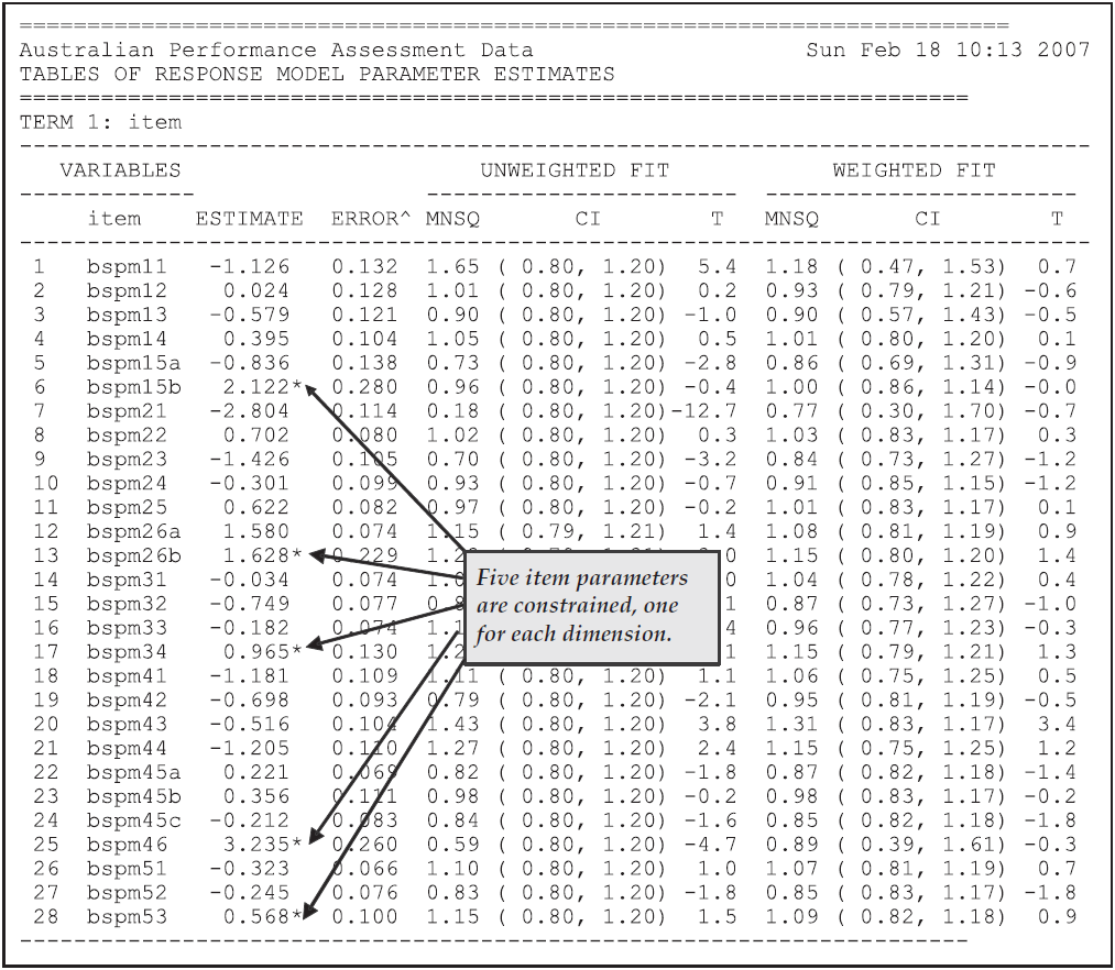
Figure 2.61: Item Parameter Estimates for a Five-Dimensional Sample Analysis

EXTENSION: As an alternative to identifying the model by making the mean of the item parameters on each dimension zero (default behaviour), the lconstraints=cases argument of the set command can be used to have the mean of each latent dimension set to zero as an alternative constraint. If this were done, all item parameters would be estimated, but the mean of each of the latent dimensions would be zero.

Figure 2.62 shows the population parameter estimates, which in this case consist of means for each of the dimensions and the five-by-five variance-covariance matrix of the latent dimensions.

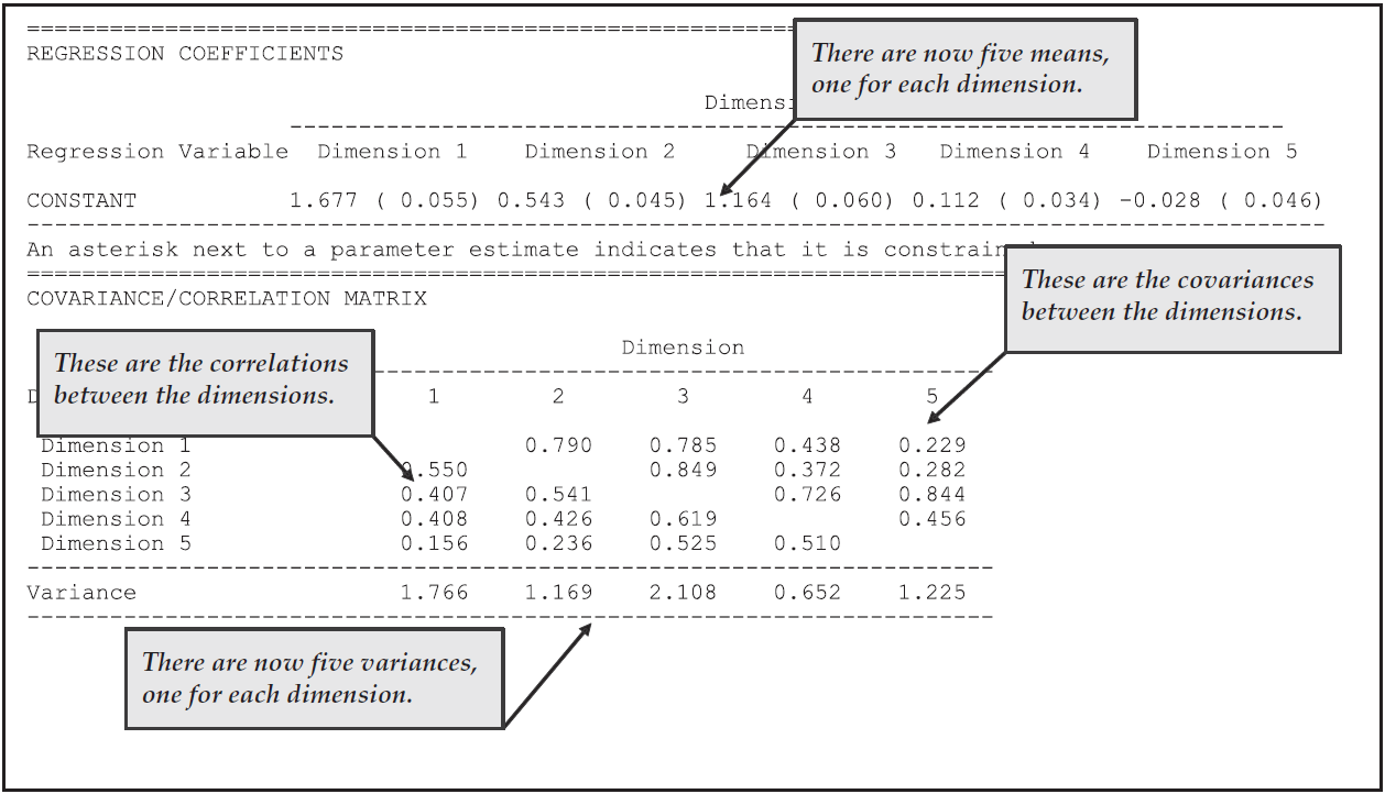
Figure 2.62: Population Model Parameter Estimates for the Five-Dimensional Sample Analysis

Figure 2.63 is a map of the five latent dimensions and the item difficulties. For the purposes of this figure, we have omitted the rightmost panel, which shows the item step-parameter estimates.

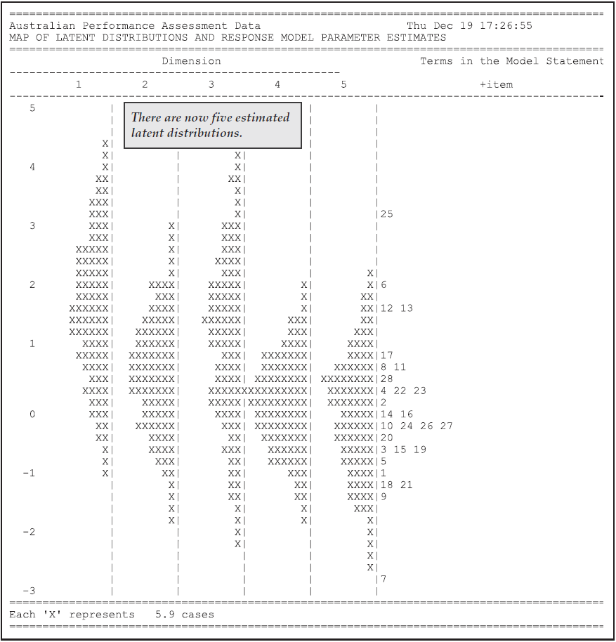
Figure 2.63: Variable Map for the Five-Dimensional Sample Analysis

2.8.3 Within-Item and Between-Item Multidimensionality

The two preceding sample analyses in this section are examples of what Wang (1995) would call between-item multidimensionality (see also Adams, Wilson, & Wang (1997)). To assist in the discussion of different types of multidimensional models and tests, Wang introduced the notions of within-item and between-item multidimensionality. A test is regarded as multidimensional between-item if it is made up of several unidimensional subscales. A test is considered multidimensional within-item if any of the items relates to more than one latent dimension.

Multidimensional Between-Item Models
Tests that contain several subscales, each measuring related but distinct latent dimensions, are very commonly encountered in practice. In such tests, each item belongs to only one particular subscale, and there are no items in common across the subscales. In the past, item response modelling of such tests has proceeded by either applying a unidimensional model to each of the scales separately or by ignoring the multidimensionality and treating the test as unidimensional. Both of these methods have weaknesses that make them less desirable than undertaking a joint, multidimensional calibration (Adams, Wilson, & Wang, 1997). In the preceding sample analyses in this section, we have illustrated the alternative approach of fitting a multidimensional model to the data.

Multidimensional Within-Item Models
If the items in a test measure more than one latent dimension and some of the items require abilities from more than one dimension, then we call the test within-item multidimensional.

The distinction between the within-item and between-item multidimensional models is illustrated in Figure 2.64.

In the left of Figure 2.64, we have depicted a between-item multidimensional test that consists of nine items measuring three latent dimensions. On the right of Figure 2.64, we have depicted a within-item multidimensional test with nine items and three latent dimensions.

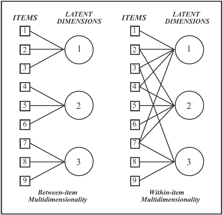
Figure 2.64: A Graphical Representation of Within-Item and Between-Item Multidimensionality

2.8.4 Example C: A Within-Item Multidimensional Model

As a final sample analysis in this section, we show how ACER ConQuest can be used to estimate a within-item multidimensional model like that illustrated in Figure 2.64.

For the purpose of this sample analysis, we use simulated data that consist of the responses of 2000 students to nine dichotomous questions. These items are assumed to assess three different latent abilities, with the relationship between the items and the latent abilities as depicted in Figure 2.64. The generating value for the mean for each of the latent abilities was zero, and the generating covariance between the latent dimensions was:

\[ \sum= \left[\begin{array}{ccc} 1.00 & 0.00 & 0.58 \\ 0.00 & 1.00 & 0.58 \\ 0.58 & 0.58 & 1.00 \end{array}\right] \]

The generating item difficulty parameters were –0.5 for items 1, 4 and 7; 0.0 for items 2, 5 and 8; and 0.5 for items 3, 6 and 9.

2.8.4.1 Required files

The files that we use in this sample analysis are:

filename	content
ex7c.cqc	The command statements used to fit the model.
ex7c_dat.txt	The data.
ex7c_prm.txt	Item parameter estimates.
ex7c_reg.txt	Regression coefficient estimates.
ex7c_cov.txt	Covariance parameter estimates.
ex7c_shw.txt	Selected results of the analysis.

2.8.4.2 Syntax

ex7c.cqc is the command file necessary for fitting the Within-Item Multidimensional Model. It is shown in the code block below, and commented upon in the list underneath the embedded command file.

This command file actually runs two analyses. The first is used to obtain an approximate solution that is used as initial values for the second analysis, which is used to produce a more accurate solution.

ex7c.cqc:

datafile ex7c_dat.txt;
format responses 1-9;
set lconstraints=cases,update=yes,warnings=no;
score (0,1) (0,1) (   ) (   ) ! items(1);
score (0,1) (0,1) (0,1) (   ) ! items(2);
score (0,1) (0,1) (   ) (0,1) ! items(3);
score (0,1) (0,1) (0,1) (   ) ! items(4);
score (0,1) (   ) (0,1) (   ) ! items(5);
score (0,1) (   ) (0,1) (   ) ! items(6);
score (0,1) (0,1) (0,1) (0,1) ! items(7);
score (0,1) (   ) (   ) (0,1) ! items(8);
score (0,1) (   ) (   ) (0,1) ! items(9);
model items;
export parameters >> ex7c_prm.txt;
export reg_coefficients >> ex7c_reg.txt;
export covariance >> ex7c_cov.txt;
estimate !method=montecarlo,nodes=200,conv=.01,fit=no,stderr=none;
reset;
datafile ex7c_dat.txt;
format responses 1-9;
set lconstraints=cases,update=yes,warnings=no;
score (0,1) (0,1) (   ) (   ) ! items(1);
score (0,1) (0,1) (0,1) (   ) ! items(2);
score (0,1) (0,1) (   ) (0,1) ! items(3);
score (0,1) (0,1) (0,1) (   ) ! items(4);
score (0,1) (   ) (0,1) (   ) ! items(5);
score (0,1) (   ) (0,1) (   ) ! items(6);
score (0,1) (0,1) (0,1) (0,1) ! items(7);
score (0,1) (   ) (   ) (0,1) ! items(8);
score (0,1) (   ) (   ) (0,1) ! items(9);
model items;
import init_parameters << ex7c_prm.txt;
import init_reg_coefficients << ex7c_reg.txt;
import init_covariance << ex7c_cov.txt;
export parameters >> ex7c_prm.txt;
export reg_coefficients >> ex7c_reg.txt;
export covariance >> ex7c_cov.txt;
estimate !method=montecarlo,nodes=1000;
show !tables=1:2:3 >> Results/ex7c_shw.txt;

Line 1
Read data from the file ex7c_dat.txt.
Line 2
The responses are in columns 1 through 9.
Line 3
Set update to yes and warnings to no so that current parameter estimates are written to a file at every iteration. This statement also sets lconstraints=cases, which should be used if ACER ConQuest is being used to estimate models that have within-item multidimensionality.

EXTENSION: ACER ConQuest can be used to estimate within-item multidimensional models without the use of lconstraints=cases. This will, however, require the user to define his or her own design matrices. A description of how to construct design matrices is found in section 2.10, Importing Design Matrices. Sample analyses that use user-defined design matrices are provided in section 3.1.7, Design Matrices.

Lines 4-12
These score statements describe how the items ‘load’ on each of the latent dimensions. The first item, for example, has scores on dimension one but not dimensions two or three. The second item is scored on the first and second dimensions, the third on the first and third, and so on.
Line 13
The items are all dichotomous, so we are using the simple logistic model.
Lines 14-16
The item, regression and covariance parameter estimates will each be written to a file. The combination of the update argument in the set statement (line 3) and these export statements means that these files will be updated at every iteration.

NOTE: The implicit variable names item and items are synonymous in ACER ConQuest, so you may use either in ACER ConQuest statements.
Line 17
In this estimation, we are using the Monte Carlo integration method with 200 nodes and a convergence criterion of 0.01. This analysis is undertaken to provide initial values for the more accurate analysis that follows.
Line 18
Resets all system values so that a new analysis can be undertaken.
Lines 19-31
As for lines 1 through 13.
Lines 32-34
Initial values for all of the parameter estimates are read from the files that were created in the previous analysis.
Lines 35-37
As for lines 14 through 16.
Line 38
The Monte Carlo method of estimation is used with 1000 nodes and the default convergence criterion of 0.001.
Line 39
Tables 1, 2 and 3 are written to ex7c_shw.txt.

2.8.4.3 Running the Within-Item Multidimensional Sample Analysis

To run this sample analysis, launch the console version of ACER ConQuest by typing the command (on Windows) ConQuestConsole.exe ex7c.cqc.

ACER ConQuest will begin executing the statements that are in the file ex7c.cqc; and as they are executed, they will be echoed on the screen. When ACER ConQuest reaches the estimate statement, it will begin fitting a within-item three-dimensional form of Rasch’s simple logistic model to the data, using 200 nodes and a convergence criterion of 0.01 with the Monte Carlo method. ACER ConQuest will then proceed to the second analysis. This analysis begins with the provisional estimates provided by the first analysis and uses 1000 nodes with the default convergence criterion of 0.0001. The show statement at the end of the command file will produce three output tables. The second and third of these are reproduced in Figures 2.65 and 2.66. The results in these tables show that ACER ConQuest has done a good job in recovering the generating values for the parameters.

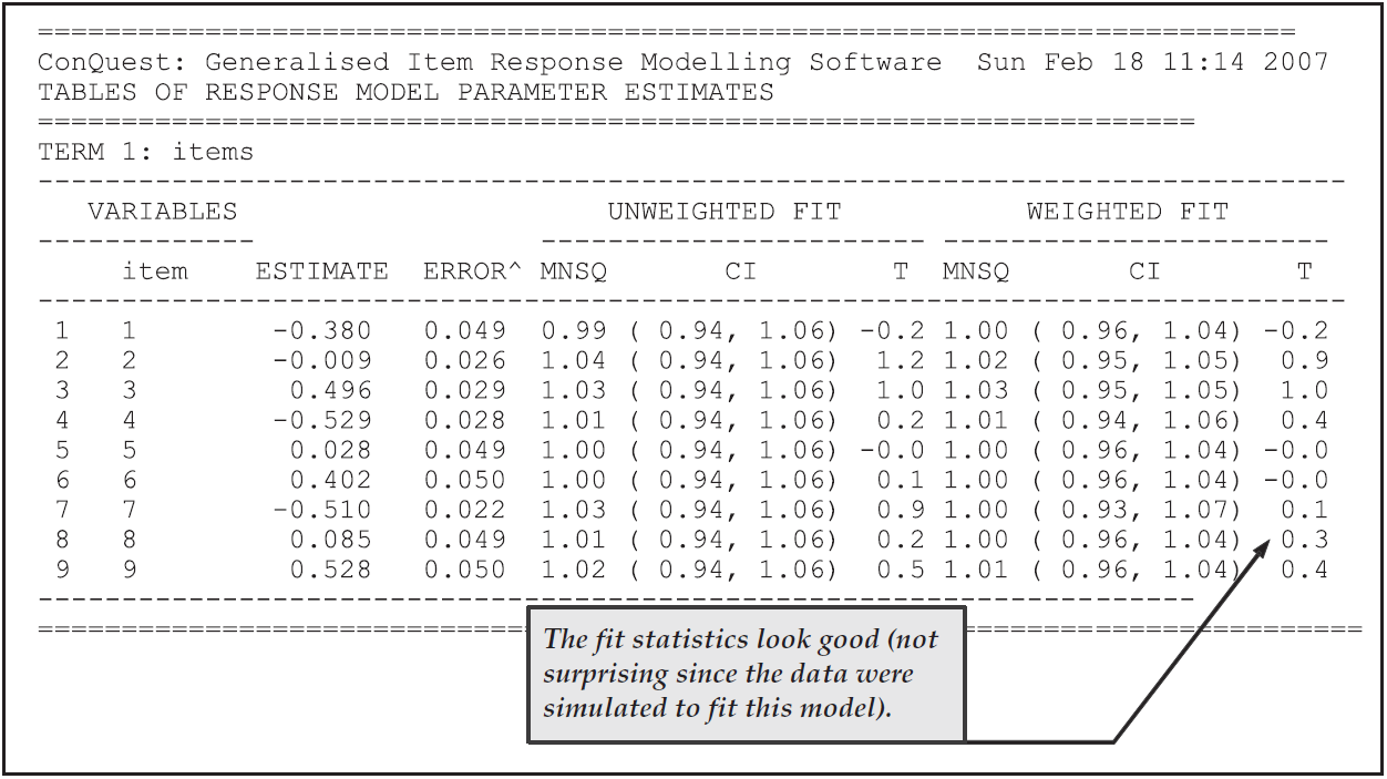
Figure 2.65: Item Parameter Estimates for a Within-Item Three-Dimensional Sample Analysis

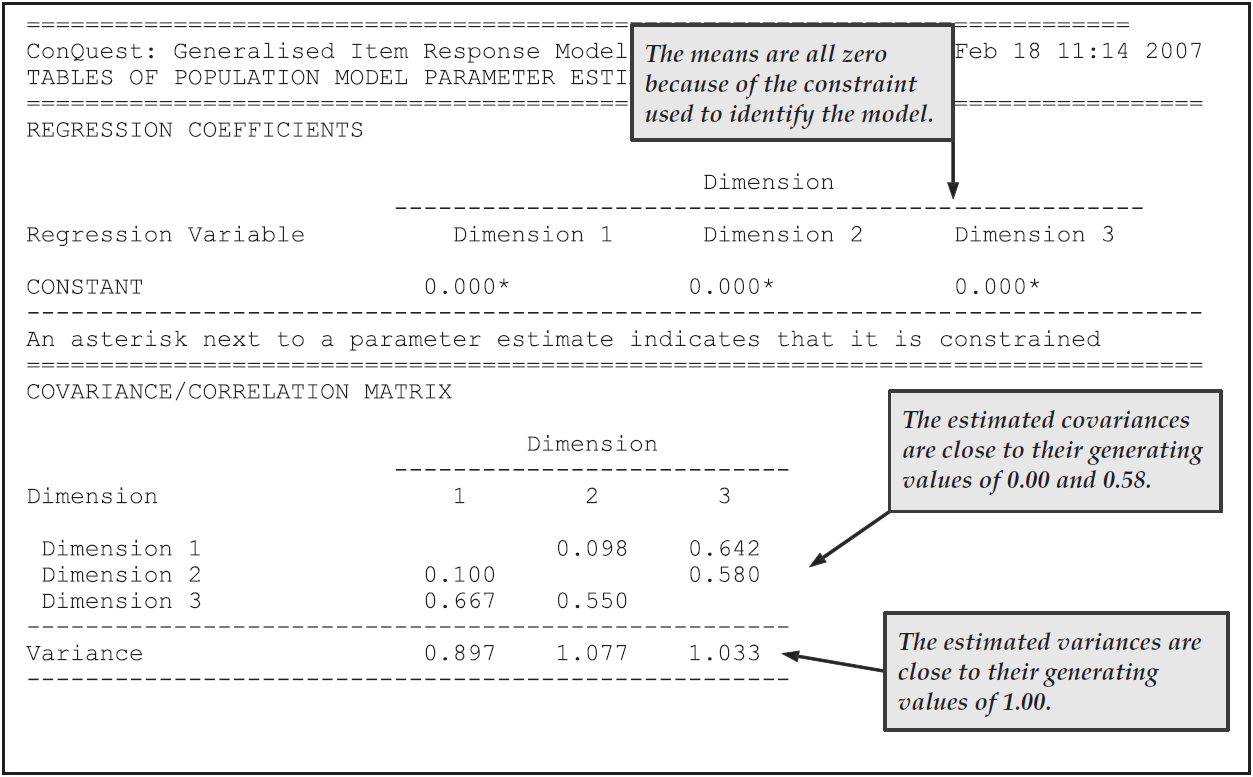
Figure 2.66: Population Parameter Estimates for a Within-Item Three-Dimensional Sample Analysis

2.8.5 Summary

In this section, we have seen how ACER ConQuest can be used to fit multidimensional item response models. Models of two, three and five dimensions have been fit.

Some key points covered in this section are:

The score statement can be used to indicate that a multidimensional item response model should be fit to the data.
The fitting of a multidimensional model as an alternative to a unidimensional model can be used as an explicit test of the fit of data to a unidimensional item response model.
The secondary analysis of latent ability estimates does not produce results that are equivalent to the ‘correct’ latent regression results. The errors that can be made in a secondary analysis of latent ability estimates are greater when measurement error is large.
ACER ConQuest offers two approximation methods, quadrature and Monte Carlo, for computing the integrals that must be computed in marginal maximum likelihood estimation. The quadrature method is generally the preferred approach for problems of three or fewer dimensions, while the Monte Carlo method is preferred for higher dimensions.
ACER ConQuest can be used to fit models that are multidimensional between-item or multidimensional within-item. Fitting multidimensional within-items requires the use of lconstraints=cases, unless an imported design matrix is used.

2.9 Multidimensional Latent Regression

In section 2.8, we illustrated how ACER ConQuest can be used to fit multidimensional item response models; and in section 2.6, we illustrated how ACER ConQuest can be used to estimate latent regression models. In this section, we bring these two functions together, using ACER ConQuest to fit multidimensional latent regression models.

In parts a) and b) of this section, we fit multidimensional latent regression models of two and five dimensions. Some output that is standard for regression analysis is not available in this version of ACER ConQuest; but in part c) we illustrate how plausible values can be drawn. The plausible values can be analysed, using traditional regression techniques, to produce further regression statistics.

The data we are analysing were collected by Adams et al. (1991) as part of their study of science achievement in Victorian schools. In their study, Adams et al. used a battery of multiple choice and extended response written tests.

The data set contains the responses of 2564 students to the battery of tests; all of the items have been prescored. The multiple choice items are located in columns 50 through 114, and the extended response test that we will use is located in columns 1 through 9. If students were administered a test but did not respond to an item, a code of 9 has been entered into the file. If a student was not administered an item, then the file contains a blank character. We will be treating the 9 as an incorrect response and the blanks as missing-response data. The student’s grade code is located in column 118, the gender code is located in column 119, and the indicator of socio-economic status is in columns 122 through 127.²⁵ The gender variable is coded 0 for female and 1 for male, the grade variable is coded 1 for the lower grade and 2 for the upper grade, and the socio-economic indicator is a composite that represents a student’s socio-economic status.

2.9.1 a) Fitting a Two-Dimensional Latent Regression

In this sample analysis, we will consider ability as assessed by the multiple choice test as one latent outcome and ability as assessed by the first of the extended response tests as a second latent outcome. Then we will regress these two outcomes onto three background variables: student grade, student gender and an indicator of socio-economic status.

2.9.1.1 Required files

The files that will be used in this sample analysis are:

filename	content
ex8a.cqc	The command statements that we use.
ex8a_no_regressors.cqc	The command statements to estimate the variance of latent variables.
ex6_dat.txt	The data.
ex8a_prm.txt	An initial set of item parameter estimates.
ex8a_reg.txt	An initial set of regression coefficient estimates.
ex8a_cov.txt	An initial set of variance-covariance parameter estimates.
ex8a_shw.txt	The population model parameter estimates.

2.9.1.2 Syntax

This sample analysis uses the command file ex8a.cqc to conduct a Two-Dimensional Latent Regression. ex8a.cqc is shown in the code box below, and explained line-by-line in the list underneath the figure.

ex8a.cqc:

datafile ex6_dat.txt;
format responses 1-9,50-114 grade 118 gender 119 ses 122-127!tasks(74);
model tasks+tasks*step;
recode (9) (0);
score (0,1,2,3,4) (0,1,2,3,4) ( ) !tasks(1-9);
score (0,1,2,3,4) ( ) (0,1,2,3,4) !tasks(10-74);
regression grade,gender,ses;
export parameters >> ex8a_prm.txt;
export reg_coefficients >> ex8a_reg.txt;
export covariance >> ex8a_cov.txt;
import init_parameters << ex8a_prm.txt;
import init_reg_coefficients << ex8a_reg.txt;
import init_covariance << ex8a_cov.txt;
set update=yes,warnings=no;
estimate!fit=no,converge=.002,stderr=quick;
show ! tables=3 >> Results/ex8a_shw.txt;

Line 1
We are analysing data in the file ex6_dat.txt.
Line 2
The format statement is reading 74 responses; assigning the label tasks to those responses; and reading grade, gender and ses data. The column specifications for the responses are made up of two separate response blocks. The first nine items are read from columns 1 through 9 (these are the extended response items that we are using), and the remaining 65 items are read from columns 50 through 114 (these are the multiple choice items).
Line 3
We are using the partial credit model because the items are a mixture of polytomous and dichotomous items.
Line 4
A code of 9 has been used for missing-response data caused by the student not responding to an item. We want to treat this as though it were identical to an incorrect response, so we recode it to 0.
Lines 5-6
We use two score statements, one for each dimension. The first statement scores the first nine tasks on the first dimension, and the second statement scores the remaining 65 tasks on the second dimension.
Line 7
This regression statement specifies a population model that regresses the two latent variables onto grade, gender and ses.
Lines 8-10
These export statements result in the parameter estimates being written to the files ex8a_prm.txt, ex8a_reg.txt and ex8a_cov.txt. In conjunction with the set statement (line 14), these export statements result in updated parameter estimates being written to these files after each iteration.
Lines 11-13
Initial values of all parameter estimates are read from the files ex8a_prm.txt, ex8a_reg.txt and ex8a_cov.txt. These initial values have been provided to speed up the analyses.
Line 14
In conjunction with the export statements (lines 8 through 10), this set statement results in updated parameter estimates being written to the files after each iteration, and it turns off warning messages.
Line 15
Begins estimation of the model. The options turn off calculation of the fit tests and instruct estimation to terminate when the change in the parameter estimates from one iteration to the next is less than 0.002.
Line 16
Writes the estimates of the population model parameter estimates to ex8a_shw.txt.

2.9.1.3 Running the Two-Dimensional Latent Regression

To run this sample analysis, launch the console version of ACER ConQuest by typing the command (on Windows) ConQuestConsole.exe ex8a.cqc.

ACER ConQuest will begin executing the statements that are in the file ex8a.cqc; and as they are executed, they will be echoed on the screen. When ACER ConQuest reaches the estimate statement, it will begin fitting the two-dimensional latent multiple regression. This particular sample analysis will converge after a single iteration, because we have provided very accurate initial values.

NOTE: If you run this sample analysis without the initial values, it will take in excess of 1000 iterations to converge. While fitting multidimensional models can take a substantial amount of computing time, this particular analysis will take an unusually large number of iterations because of the sparse nature of the data set. In these data, just 40% of the students responded to items on the first dimension; and the first 50 multiple choice items were responded to by only 25% of the sample. All students responded to the last 15 items.

In Figure 2.67, we report the parameter estimates for the population model used in this analysis. In this case, we have two sets of four regression coefficients — a constant and one for each of the three regressors. The conditional variance-covariance matrix is also reported.

All of the results reported here are in their natural metrics (logits). For example, on the first dimension, the difference between the performances of the lower grade and upper grades is 0.700 logits, the male students outperform the female students by 0.072, and a unit increase in the socio-economic status indicator predicts an increase of 0.366 logits in the latent variable. For the second dimension, the difference between the performances of the lower grade and upper grades is 1.391 logits, the male students outperform the female students by 0.229, and a unit increase in the socio-economic status indicator predicts an increase of 0.479 logits in the latent variable.²⁶

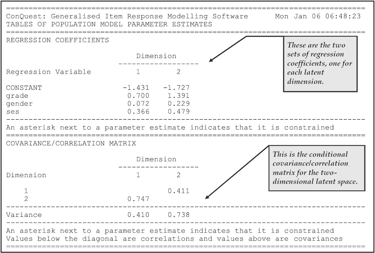
Figure 2.67: Population Parameter Estimates for a Two-Dimensional Latent Multiple Regression

To aid in the interpretation of these results, it is useful to fit a model without the regressors to obtain estimates of the variance of the two latent variables in this model, the multiple choice items and the extended response item. The command file ex8a_no_regressors.cqc is provided with the samples for this purpose. If this command file is executed, it will provide estimates of 0.601 (extended response) and 1.348 (multiple choice) for the variances of the two latent variables.

In Figure 2.68, we report the \(R^2\) for each of the dimensions in the latent regression, and we report the grade, gender and socio-economic status (SES) regression coefficients as effect sizes that have been computed by dividing the estimate of the regression coefficients by the unconditional standard deviation of the respective latent variables.

The results in the table show that the regression model explains marginally more variance for the multiple choice items than it does for the extended response items. Interestingly, the grade and SES effects are similar for the item types, but the gender effect is larger for the multiple choice items. For the extended response items, the gender difference is 9% of a student standard deviation, whereas for the multiple choice it is 19.7%.

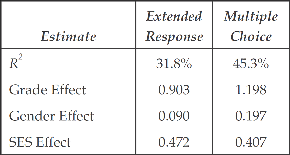
Figure 2.68: Effect Size Estimates for the Two-Dimensional Latent Multiple Regression

EXTENSION: The model fitted in ex8b.cqc has the item response model parameters anchored at the values that were obtained from the model that is fit with ex8a.cqc. In general, the item response parameter estimates obtained from fitting a model with regressors will produce item parameter estimates that have smaller standard errors, although the gain in efficiency is generally very small. More importantly, there are occasions when item response model parameters estimated without the use of regressors will be inconsistent. This data set provides such a case, because some of the multiple choice items were administered only to students in the upper grade, while others were administered only to students in the lower grade. Readers interested in this issue are referred to Mislevy & Sheehan (1989) and Adams, Wilson, & Wu (1997).

2.9.2 b) Five-Dimensional Multiple Regression - Unconditional Model

In the Adams et al. (1991) battery of tests, four extended response tests and a set of 15 multiple choice were administered to students in both the upper and lower grades. In this higher-dimensional sample analysis, we are interested in grade, gender and SES effects for the five latent dimensions that are assumed to be assessed by these instruments. First, we will run an unconditional model (using the command file ex8b.cqc, described in Section 2.9.2.1) to obtain initial values for a conditional model. Then we will run the conditional model and will also have ACER ConQuest draw plausible values, using the command file ex8c.cqc (shown in Section 2.9.3.1).

Because of the high dimensionality, the analysis that is required here is best undertaken with Monte Carlo integration; and as this will need a large number of nodes, the model without regressors (the unconditional model) is fitted in two stages. In the first stage, a small number of nodes with a moderate convergence criterion is used to produce initial values. In the second stage, the initial values are read back into an analysis that uses more nodes and a more stringent convergence criteria.

2.9.2.1 Syntax

The contents of the command file for this tutorial (ex8b.cqc), are shown in the code box located below. ex8b.cqc is used to fit the Five-Dimensional Latent Unconditional Model to the dataset ex6_dat.txt. The list underneath the code box describes each line of syntax.

ex8b.cqc:

datafile ex6_dat.txt;
format responses 1-18,31-49,100-114 grade 118 gender 119 ses 122-127
        !tasks(52);
model tasks+tasks*step;
recode (9) (0);
score (0,1,2,3,4) (0,1,2,3,4) ( ) ( ) ( ) ( ) ! tasks(1-9);
score (0,1,2,3,4) ( ) (0,1,2,3,4) ( ) ( ) ( ) ! tasks(10-18);
score (0,1,2,3,4) ( ) ( ) (0,1,2,3,4) ( ) ( ) ! tasks(19-28);
score (0,1,2,3,4) ( ) ( ) ( ) (0,1,2,3,4) ( ) ! tasks(29-37);
score (0,1,2,3,4) ( ) ( ) ( ) ( ) (0,1,2,3,4) ! tasks(38-52);
export reg_coefficient >> ex8b_reg.txt;
export covariance >> ex8b_cov.txt;
export parameters >> ex8b_prm.txt;
set update=yes,warnings=no;
estimate!fit=no,method=montecarlo,nodes=400,conv=.01,stderr=none;
reset;
datafile ex6_dat.txt;
format responses 1-18,31-49,100-114 grade 118 gender 119 ses 122-127
        !tasks(52);
model tasks+tasks*step;
recode (9) (0);
score (0,1,2,3,4) (0,1,2,3,4) ( ) ( ) ( ) ( ) ! tasks(1-9);
score (0,1,2,3,4) ( ) (0,1,2,3,4) ( ) ( ) ( ) ! tasks(10-18);
score (0,1,2,3,4) ( ) ( ) (0,1,2,3,4) ( ) ( ) ! tasks(19-28);
score (0,1,2,3,4) ( ) ( ) ( ) (0,1,2,3,4) ( ) ! tasks(29-37);
score (0,1,2,3,4) ( ) ( ) ( ) ( ) (0,1,2,3,4) ! tasks(38-52);
export parameters >> ex8b_prm.txt;
import init_reg_coefficient << ex8b_reg.txt;
import init_covariance << ex8b_cov.txt;
import init_parameters << ex8b_prm.txt;
set update=yes,warnings=no;
estimate!method=montecarlo,nodes=2000,conv=.002,stderr=quick;
show !tables=1:3:5 >> Results/ex8b_shw.txt;

Line 1
We are using the data in ex6_dat.txt.
Lines 2-3
The responses to the four extended response instruments administered to all the students are in columns 1 through 18 and 31 through 49; and the responses to the 15 multiple choice items administered to all the students are in columns 100 through 114. Columns 19 through 30 contain the responses to an instrument that was administered to the lower grade students only, and columns 50 through 99 contain the responses to multiple choice items that were administered to students in one of the grades only. We have decided not to include those data in these analyses.
Line 4
We are using the partial credit model.
Line 5
Any code of 9 (item not responded to by the student) will be recoded to 0 and therefore scored as 0.
Lines 6-10
These five score statements allocate the items that make up the five instruments to the five different dimensions.
Lines 11-14
The export statements, in conjunction with the set statement, ensure that the parameter estimates are written to the files ex8b_reg.txt, ex8b_cov.txt and ex8b_prm.txt after each iteration. This is useful if you want to use the values generated by the final iteration as initial values in a further analysis, as we will do here.
Line 15
Initiates the estimation of a partial credit model using the Monte Carlo method to approximate multidimensional integrals. This estimation is done with 400 nodes, a value that will probably lead to good estimates of the item parameters, but the latent variance-covariance matrix may not be well estimated.²⁷ We are using 400 nodes here to obtain initial values for input into the second analysis that uses 2000 nodes. We have specified fit=no because we will not be generating any displays and thus have no need for this data at this time. We are also using a convergence criteria of just 0.01, which is appropriate for the first stage of a two-stage estimation.
Line 16
The reset statement resets all variables to their initial values and is used to separate distinct analyses that are in a single command file.
Lines 17-26
As for lines 1 through 10 above.
Line 27
We are exporting only the item response model parameter estimates.
Lines 28-30
Initial values for all of the parameter estimates are being read from the files that were written in the previous analysis.
Line 31
Used in conjunction with line 27 to ensure that the item response model parameter estimates are written after each iteration.
Line 32
The estimation method is Monte Carlo, but this time we are using 2000 nodes and a convergence criterion of 0.002. This should be sufficient to produce accurate estimates for all of the parameters.
Line 33
Writes selected tables to the output file ex8b_shw.txt.

2.9.2.2 Running the Five-Dimensional Latent Unconditional Sample Analysis

To run this sample analysis, launch the console version of ACER ConQuest by typing the command (on Windows) ConQuestConsole.exe ex8b.cqc.

ACER ConQuest will begin executing the statements in the file ex8b.cqc; and as they are executed, they will be echoed on the screen. When ACER ConQuest reaches the first estimate statement, it will begin fitting the five-dimensional model using a 400-node Monte Carlo integration. ACER ConQuest will then proceed to analyse the data again using a 2000-node Monte Carlo integration, reading initial values from the export files produced by the previous 400-node analysis.

Figure 2.69 shows the estimated population parameters for the unconditional fivedimensional latent space. The analysis shows that the correlation between these latent dimensions is moderately high but unlikely to be high enough to justify the use of a unidimensional model.

NOTE: If you run this sample analysis without the initial values, it will take in excess of 1000 iterations to converge. While fitting multidimensional models can take a substantial amount of computing time, this particular analysis will take an unusually large number of iterations because of the sparse nature of the data set. In these data, just 40% of the students responded to items on the first dimension; and the first 50 multiple choice items were responded to by only 25% of the sample. All students responded to the last 15 items.

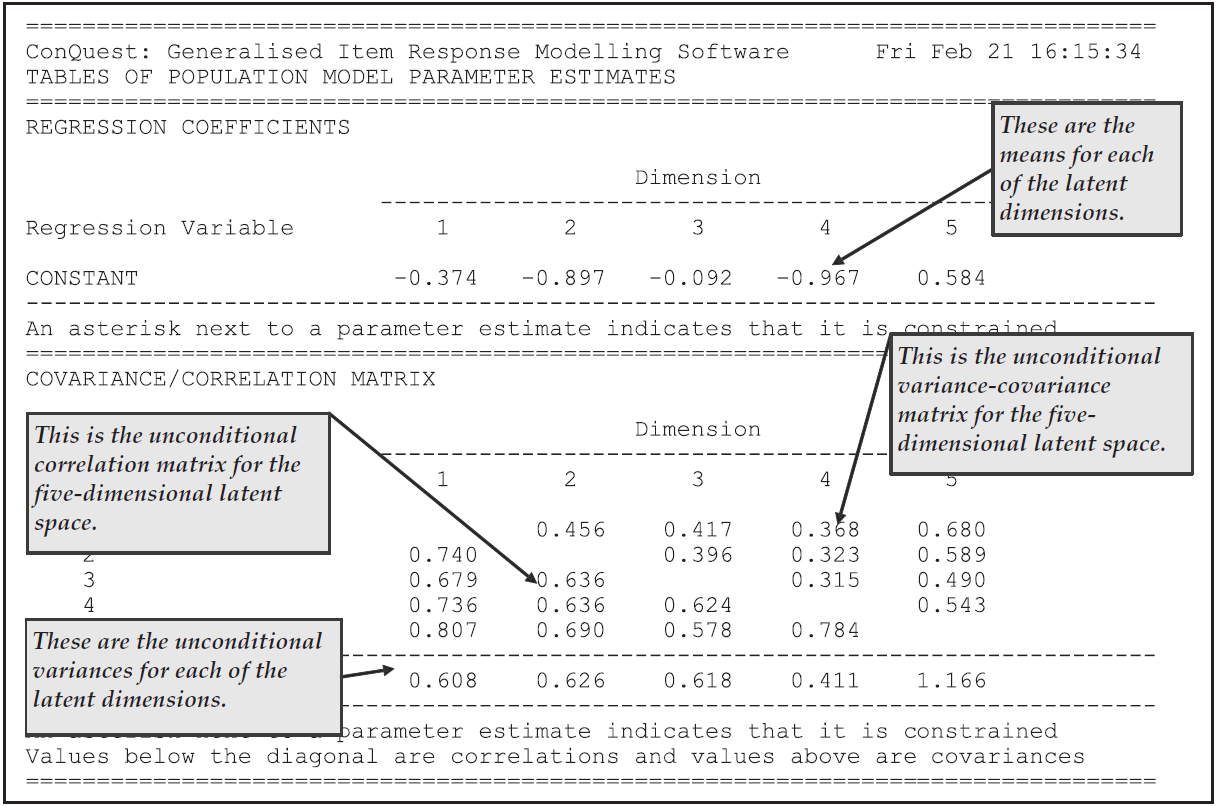
Figure 2.69: Population Parameter Estimates for the Unconditional Five-Dimensional Model

2.9.3 c) Five-Dimensional Multiple Regression - Conditional Model

2.9.3.1 Syntax

ex8c.cqc is the command file for fitting the five-dimensional latent regression model (the conditional model). It is given in the code box below. ex8c.cqc is very similar to the command file used for the unconditional analysis (ex8b.cqc, see Section 2.9.2.1). So the description of ex8c.cqc underneath the code embedding will focus only on the differences.

ex8c.cqc:

datafile ex6_dat.txt;
format responses 1-18,31-49,100-114 grade 118 gender 119 ses 122-127!tasks(52);
regression grade,gender,ses;
model tasks+tasks*step;
recode (9) (0);
score (0,1,2,3,4) (0,1,2,3,4) ( ) ( ) ( ) ( ) ! tasks(1-9);
score (0,1,2,3,4) ( ) (0,1,2,3,4) ( ) ( ) ( ) ! tasks(10-18);
score (0,1,2,3,4) ( ) ( ) (0,1,2,3,4) ( ) ( ) ! tasks(19-28);
score (0,1,2,3,4) ( ) ( ) ( ) (0,1,2,3,4) ( ) ! tasks(29-37);
score (0,1,2,3,4) ( ) ( ) ( ) ( ) (0,1,2,3,4) ! tasks(38-52);
import init_covariance <<ex8b_cov.txt;
import anchor_parameters <<ex8b_prm.txt;
estimate!method=montecarlo,nodes=2000,conv=.002,iter=3,stderr=quick;
show cases !estimates=latent >> Results/ex8c_pls.txt;
show cases !estimates=eap >> Results/ex8c_eap.txt;
show !tables=1:3:5>> Results/ex8c_shw.txt;

Line 3
The third statement in this command file specifies the regression variables that are to be used in the model (in this case, grade, gender and ses).
Line 11
This import statement uses the estimated unconditional variance-covariance matrix as an initial value. This is done in this sample analysis so that the analysis will be performed more quickly.
Line 12
This import statement requests that item response model parameter values be read from the file ex8b_prm.txt (created by the five-dimensional unconditional model) and be anchored at the values specified in that file. This means that, in this analysis, we will not be estimating item parameters.

WARNING: The current version of ACER ConQuest is unable to estimate both item response model parameters and population model parameters in a conditional model (that is, a model with regressors) when the Monte Carlo method is used. This will not usually be a severe limitation because you can generally obtain consistent estimates of the item parameters by fitting an unconditional model and then entering those estimates as anchored values in a conditional model.
Line 13
The estimation will be done with the Monte Carlo method, using 2000 nodes and a convergence criterion of 0.002.
Lines 14-15
These show statements result in plausible values and expected a-posteriori estimates being written to the files ex8c_pls.txt and ex8c_eap.txt respectively.
Line 16
The final show statement requests tables 1, 3 and 5 be written to file ex8c_shw.txt.

2.9.3.2 Running the Five-Dimensional Latent Regression Sample Analysis

To run this sample analysis, launch the console version of ACER ConQuest by typing the command (on Windows) ConQuestConsole.exe ex8c.cqc.

ACER ConQuest will begin executing the statements in the file ex8c.cqc; and as they are executed, they will be echoed on the screen. When ACER ConQuest reaches the estimate statement, it will begin fitting the five-dimensional model, using a 2000-node Monte Carlo integration. The show statements will then be executed, producing files of plausible values, expected a-posteriori ability estimates and output tables. Extracts from the first two files are shown in Figures 2.70 and 2.71.

NOTE: The expected a-posteriori and plausible value files contain values for all cases on all dimensions—even for latent dimensions on which the cases have not responded to any questions. If there are dimensions for which one or more cases have not made any response, then maximum likelihood ability estimates of the latent variable cannot be calculated.

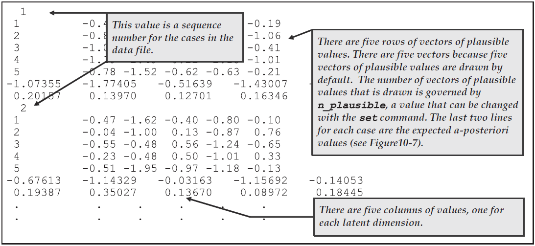
Figure 2.70: Extract from the File of Plausible Value

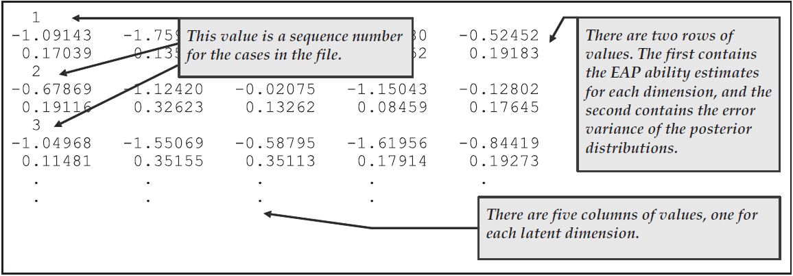
Figure 2.71: Extract from the File of Expected A-posteriori Values

²⁸

Figure 2.72 shows the estimates of the parameters of the population model. It contains estimates of the four regression coefficients for each of the latent dimensions and the estimate of the conditional variance-covariance matrix between the dimensions. This variance-covariance matrix is also expressed as a correlation matrix.

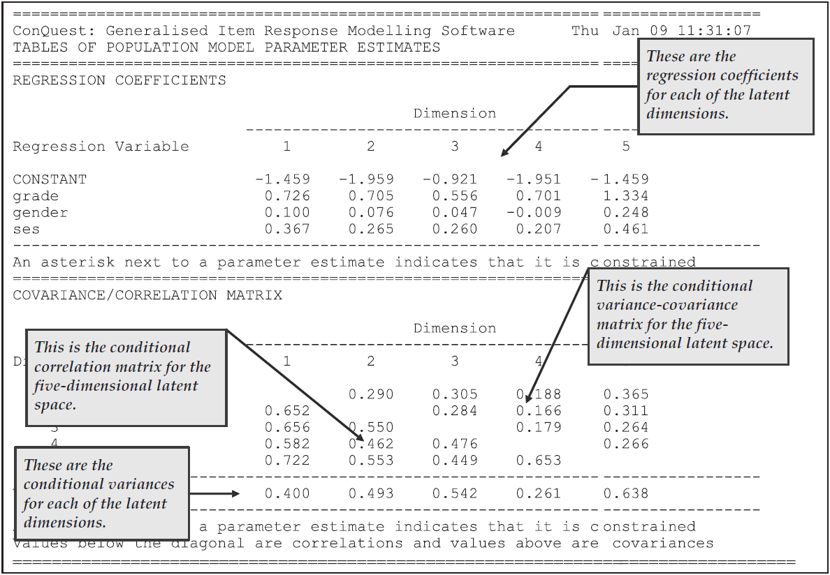
Figure 2.72: Population Model Parameter Estimates for the Five-Dimensional Latent Regression

In Figure 2.73, the estimates of the regression coefficients have been divided by the estimate of the unconditional standard deviation of the respective latent variables to provide effect size estimates. Combining the unconditional results that were obtained from analysing the data with the command file ex8b.cqc and were reported in Figure 2.69 with the latent regression results produced using the command file ex8c.cqc and reported in Figure 2.72, we obtain the effect size estimates reported in Figure 2.73. Additional analyses of this latent regression model can be obtained by merging the EAP ability estimates and the plausible values with the background variables (such as gender or grade) and undertaking conventional analyses.

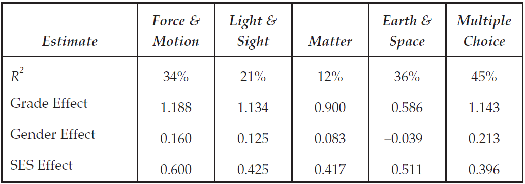
Figure 2.73: Effect Size Estimates for the Five-Dimensional Latent Multiple Regression

2.9.4 Summary

In this section, we have seen how ACER ConQuest can be used to fit multidimensional latent regression models. The fitting of multidimensional latent regression models brings together two sets of functionality that we have demonstrated in previous sections: the facility to estimate latent regression models and the facility to fit multidimensional item response models.

2.10 Importing Design Matrices

In this section, we provide sample analyses in which the model is described through a design matrix, rather than through a model statement. In each of the other sample analyses in this manual, a model statement is used to specify the form of the model, and ACER ConQuest then automatically builds the appropriate design matrix. While the model statement is very flexible and allows a diverse array of models to be specified, it does not provide access to the full generality of the model that is available when a design matrix is directly specified rather than built with a model statement.

Contexts in which the importation of design matrices are likely to be useful include:

Imposing Parameter Equality Constraints: On some occasions, you may wish to constrain the values of one or more item parameters to the same value. For example, you may want to test the hypothesis of the equality of two or more parameters.
Mixing Rating Scales: Under some circumstances, you may need to analyse a set of items that contain subsets of items, each of which use different rating scales. These subsets could be assessing the same latent variable, or they could be assessing different latent variables and a multidimensional analysis may be undertaken.
Mixing Faceted and Non-faceted Data: A set of item responses may include a mix of objectively scored items (for example, multiple choice items) and some items that required the use of raters. Under these circumstances, the rater facet would not apply to the objectively scored items.
Modelling Within-item Multidimensionality: ACER ConQuest can only automatically generate design matrices for within-item multidimensional tests if the mean of the latent variables is set to zero. Within-item multidimensional tests that do not have this constraint can, however, be analysed if a design matrix is imported.

In this section, we will provide two sample analyses in which a design matrix is imported so that a model that cannot be described by a model statement can be fitted. The first sample analysis (a)) illustrates the use of an imported design to model a mixture of two rating scales. The second (b)) shows how within-item multidimensionality without setting the means of the latent variables to zero can be accommodated.

The data we analyse in this section were collected as part of the SEPUP study (Roberts et al., 1997). It consists of the responses of 721 students to a set of 18 items that used two different rubrics. Items 1, 2, 3, 6, 10, 12, 13, 16, 17 and 18 used one rubric, and items 4, 5, 7, 8, 9, 11, 14, and 15 used an alternative rubric.

2.10.1 a) Mixing Rating Scales

In this sample analysis, we fit a sequence of three models to these data. First, we fit a rating scale model that imposes a common rating structure on all of the items. Then we use an imported design matrix to fit a model that uses two rating scales, one for the items that used the first rubric and one for the items that used the second rubric. We then fit a partial credit model.

2.10.1.1 Required files

The files used in this sample analysis are:

filename	content
ex9a.cqc	The command statements that we use.
ex9a_dat.txt	The data.
ex9a_des.txt	The design matrix imported to fit the mixture of rating scales.
ex9a_1_shw.txt	The results of the rating scale analysis.
ex9a_2_shw.txt	The results of the mixture of two rating scales.
ex9a_3_shw.txt	The results of the partial credit analysis.

2.10.1.2 Syntax

The command file used to fit the model in this section (ex9a.cqc) is shown in the code box below. In the text that follows the figure, each line of syntax is explained.

ex9a.cqc:

datafile ex9a_dat.txt;
format responses 5-9,12,15,17,18,24-32;
codes 1 2 3 4 5;
score (1 2 3 4 5) (0 1 2 3 4);
model item + step;
estimate;
show >> Results/ex9a_1_shw.txt;
reset;
datafile ex9a_dat.txt;
format responses 5-9,12,15,17,18,24-32;
codes 1 2 3 4 5;
score (1 2 3 4 5) (0 1 2 3 4);
model item + step;
import designmatrix << ex9a_des.txt;
estimate;
show >> Results/ex9a_2_shw.txt;
reset;
datafile ex9a_dat.txt;
format responses 5-9,12,15,17,18,24-32;
codes 1 2 3 4 5;
score (1 2 3 4 5) (0 1 2 3 4);
model item + item*step;
estimate;
show >> Results/ex9a_3_shw.txt;

Line 1
The data file is ex9a_dat.txt.
Line 2
The format statement describes the locations of the 18 items in the data file.
Line 3
The codes 1, 2, 3, 4 and 5 are valid.
Line 4
A score statement is used to assign scores to the codes. As this is a unidimensional analysis, a recode statement could have been used as an alternative to this score statement.
Line 5
This model statement results in a rating scale model that is applied to all items.
Line 6
Commences the estimation.
Line 7
Writes some results to the file ex9a_1_shw.txt.
Line 8
Resets all system values at their defaults so that a new analysis can be started.
Lines 9-12
As for lines 1 through 4 above.
Lines 13-14
These two lines together result in a model being fitted that uses a mixture of two rating scales. The model statement must be supplied even when a model is being imported. This model statement allows ACER ConQuest to identify the generalised items that are to be analysed with the imported model. In this case, we need ACER ConQuest to identify 18 items, so we simply use a model statement that will generate a standard rating scale model for the 18 items. The second line imports the design that is in the file ex9a_des.txt. This matrix will replace the design matrix that is automatically generated by ACER ConQuest in response to the model statement. The contents of the imported design are illustrated and described in Figure 2.74.
Lines 15-17
Estimates the model and writes results to ex9a_2_shw.txt and resets the system values.
Lines 18-24
This set of commands is the same as for lines 1 through 7, except that we are fitting a partial credit rather than a rating scale model and writing to the file ex9a_3_shw.txt.

NOTE: The number of rows in the imported design matrix must correspond to the number of rows that ACER ConQuest is expecting. ACER ConQuest determines this using a combination of the model statement and an examination of the data. The model statement indicates which combinations of facets will be used to define generalised items. ACER ConQuest then examines the data to find all of the different combinations; and for each combination, it finds the number of categories.

The best strategy for manually building a design matrix usually involves running ACER ConQuest, using a model statement to generate a design matrix, and then exporting the automatically generated matrix, using the designmatrix argument of the export statement. The exported matrix can then be edited as needed.

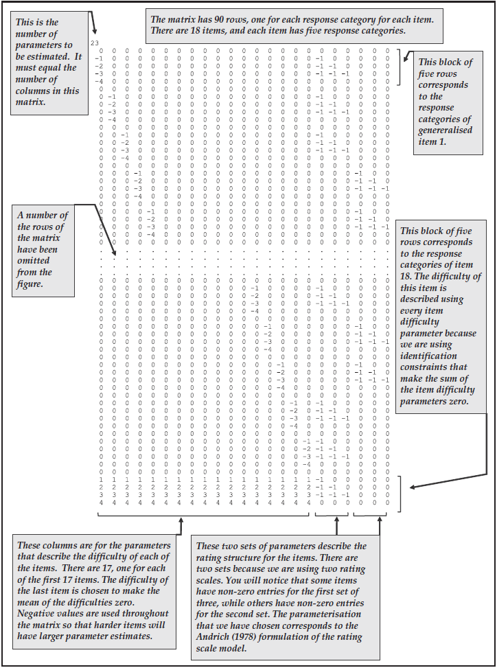
Figure 2.74: The Imported Design Matrix for Mixing Two Rating Scale

2.10.1.3 Running the Mixture of Rating Scales

To run this sample analysis, launch the console version of ACER ConQuest by typing the command (on Windows) ConQuestConsole.exe ex9a.cqc.

ACER ConQuest will begin executing the statements that are in the file ex9a.cqc; and as they are executed, they will be echoed on the screen. When ACER ConQuest reaches the first estimate statement, it will begin fitting the rating scale model to the data. The results will be written to the file ex9a_1_shw.txt. ACER ConQuest will then proceed to analyse the imported model, writing results to the file ex9a_2_shw.txt; and then the partial credit model will be fitted, writing the results to ex9a_3_shw.txt.

In Figure 2.75, the fit of this sequence of models is compared using the deviance statistic. Moving from the rating scale to the mixture improves the deviance by 50.42 and requires an additional three parameters; this is clearly significant. The improvement between the mixture and partial credit model is 160.3, and the partial credit model requires 48 additional parameters. This improvement is also significant, although the amount of improvement per parameter is considerably less than that obtained in moving from the rating scale to the mixture of two rating scales. An examination of the parameter fit statistics in the files ex9a_1_shw.txt, ex9a_2_shw.txt and ex9a_3_shw.txt leads to the same conclusions as does the examination of Figure 2.75.

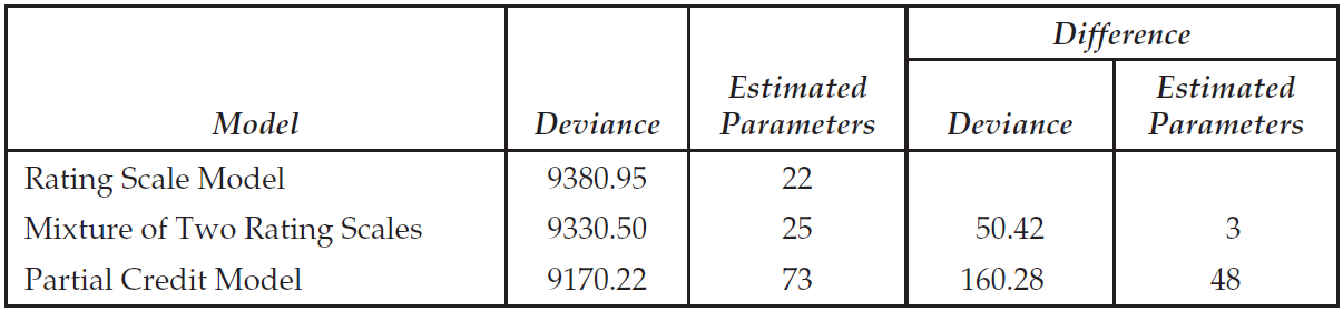
Figure 2.75: Deviance Statistics for the Three Models Fitted to the SEPUP Data

When a model is imported, the ACER ConQuest output will only be provided in an abbreviated form with all parameters listed in one Table. The output produced for the mixture of rating scales is shown in Figure 2.76.

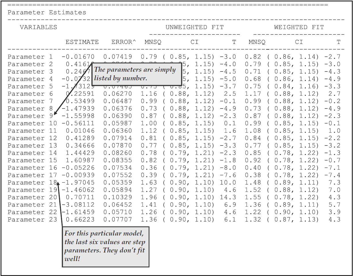
Figure 2.76: Unlabelled Output that is Produced when a Design Matrix is Imported

2.10.2 b) Within-Item Multidimensionality

As a second sample analysis that uses an imported design matrix, we will return to the within-item multidimensional sample analysis that was used in section 2.8. In section 2.8, we used lconstraints=cases, since this enabled ACER ConQuest to automatically generate a design matrix for the model. If the model is to be identified by applying constraints to the item parameters, then ACER ConQuest cannot automatically generate the design matrix for withinitem multidimensional models.²⁹

2.10.2.1 Required files

The files used in this sample analysis are:

filename	content
ex9b.cqc	The command statements.
ex7_dat.txt	The data.
ex9b_des.txt	The design matrix imported to fit the within-item multidimensional model.
ex9b_prm.txt	Initial values for the item parameter estimates.
ex9b_reg.txt	Initial values for the regression parameter estimates.
ex9b_cov.txt	Initial values for the covariance parameter estimates.
ex9b_shw.txt	The results of the rating scale analysis.

2.10.2.2 Syntax

The command file for this sample analysis is ex9b.cqc (as shown in the code box below). As this command file is very similar to ex7c.cqc (which was discussed in Section 2.8.4.2), the list below the embedded code will only highlight the differences between ex9b.cqc and ex7c.cqc.

ex9b.cqc:

datafile ex7_dat.txt;
format responses 1-9;
set update=yes,warnings=no;
score (0,1) (0,1) (   ) (   ) ! items(1);
score (0,1) (0,1) (0,1) (   ) ! items(2);
score (0,1) (0,1) (   ) (0,1) ! items(3);
score (0,1) (0,1) (0,1) (   ) ! items(4);
score (0,1) (   ) (0,1) (   ) ! items(5);
score (0,1) (   ) (0,1) (   ) ! items(6);
score (0,1) (0,1) (0,1) (0,1) ! items(7);
score (0,1) (   ) (   ) (0,1) ! items(8);
score (0,1) (   ) (   ) (0,1) ! items(9);
model items;
import designmatrix << ex9b_des.txt;
export parameters >> ex9b_prm.txt;
export reg_coefficients >> ex9b_reg.txt;
export covariance >> ex9b_cov.txt;
estimate !method=montecarlo,nodes=200,conv=.01;
reset;
datafile ex7_dat.txt;
format responses 1-9;
set update=yes,warnings=no;
score (0,1) (0,1) (   ) (   ) ! items(1);
score (0,1) (0,1) (0,1) (   ) ! items(2);
score (0,1) (0,1) (   ) (0,1) ! items(3);
score (0,1) (0,1) (0,1) (   ) ! items(4);
score (0,1) (   ) (0,1) (   ) ! items(5);
score (0,1) (   ) (0,1) (   ) ! items(6);
score (0,1) (0,1) (0,1) (0,1) ! items(7);
score (0,1) (   ) (   ) (0,1) ! items(8);
score (0,1) (   ) (   ) (0,1) ! items(9);
model items;
import designmatrix << ex9b_des.txt;
import init_parameter << ex9b_prm.txt;
import init_reg_coefficients << ex9b_reg.txt;
import init_covariance << ex9b_cov.txt;
export parameters >> ex9b_prm.txt;
export reg_coefficients >> ex9b_reg.txt;
export covariance >> ex9b_cov.txt;
estimate !method=montecarlo,nodes=1000;
show >> Results/ex9b_shw.txt;

Lines 3 & 22
Note that these set statements do not include lconstraints=cases, as did the set statements in the command file ex7c.cqc, shown in Section 2.8.4.2 (lines 3 and 21). Thus, the means for the latent dimensions will not be constrained, and identification of the model must be assured through the design for the item parameters. ACER ConQuest cannot automatically generate a correct design for a within-item multidimensional model without lconstraints=cases, so an imported design is necessary.
Lines 14 & 33
These import statements request that a user-specified design be imported from the file ex9b_des.txt to replace the design that ACER ConQuest has automatically generated.³⁰ The contents of the imported design are shown in Figure 2.77. A full explanation of how designs can be prepared for within-item multidimensional models is beyond the scope of this manual. The interested reader is referred Design Matrices in section 3.1 and to Volodin & Adams (1995).
Line 41
The show statement cannot produce individual tables when an imported design matrix is used.

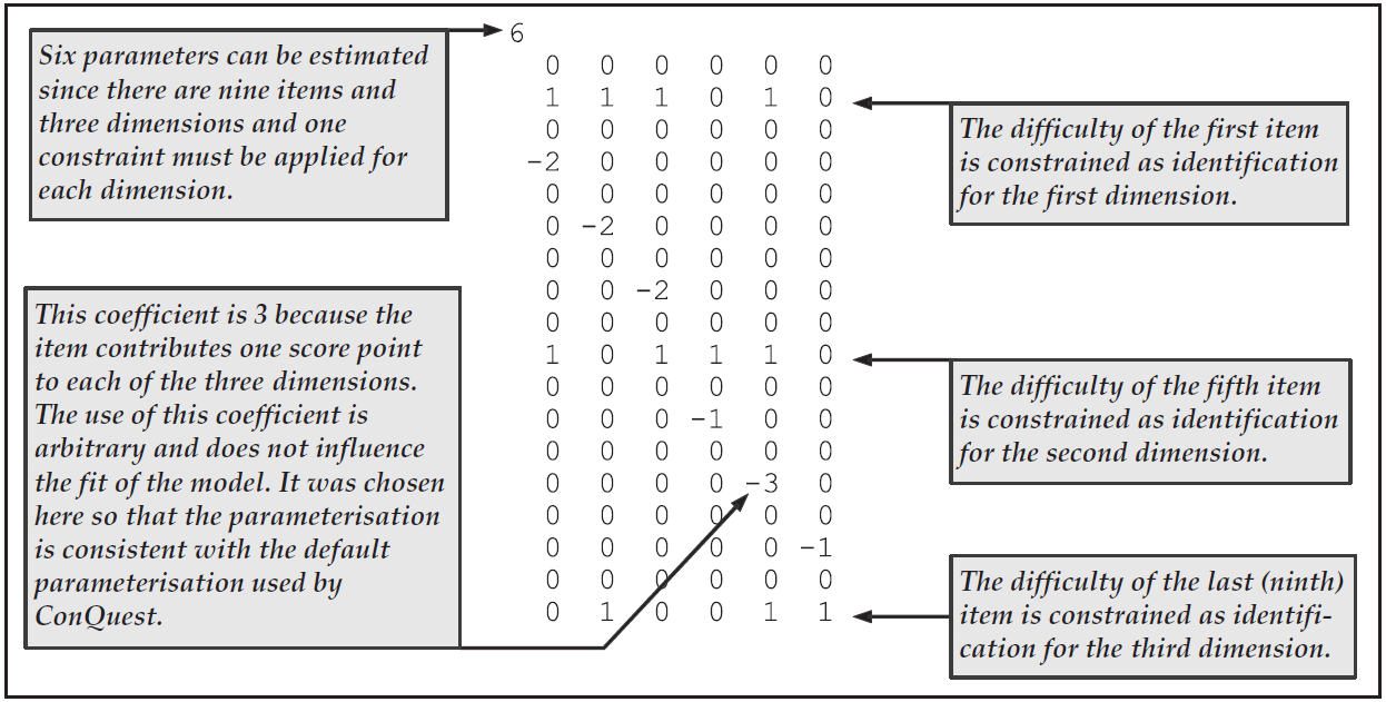
Figure 2.77: Design Matrix Used to Fit a Three-Dimensional Within-Item Model

2.10.2.3 Running the Within-Item Multidimensional Sample Analysis with an Imported Design Matrix

To run this sample analysis, launch the console version of ACER ConQuest by typing the command (on Windows) ConQuestConsole.exe ex9b.cqc.

ACER ConQuest will begin executing the statements that are in the file ex9b.cqc; and as they are executed, they will be echoed on the screen. As with the corresponding sample analysis in section 2.8, this sample analysis will fit a within-in three-dimensional form of Rasch’s simple logistic model, first approximately, using 200 nodes, and then more accurately, using 1000 nodes.

The results obtained from this analysis are shown in Figure 2.78.

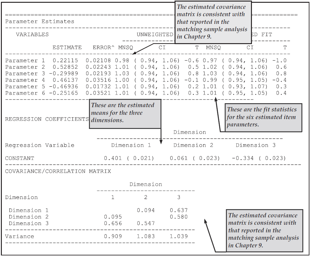
Figure 2.78: Output from the Three-Dimensional Within-Item Sample Analysis with Imported Design

EXTENSION: The multidimensional item response model given in section 3.1 is written as:

\(f(x;\xi|\theta)=\psi(\theta, \xi) \exp[x'(B\theta+A\xi)]\)

with \(\theta \sim MVN(\mu,\sum)\).

If \(\theta\) is rewritten as \(\theta^*+\mu\) with \(\theta^* \sim MVN(0,\sum)\), then it can be shown that two models, one described with the design matrices A and B and one descrived with design matrices \(A^*\) and \(B^*\), are equivalent if

\(B^*\mu^*+A^*\xi^*=B\mu+A\xi\)

A small amount of matrix algebra can be used to show that the results reported in Figures 2.65 and 2.78 satisfy this condition.

2.10.3 Summary

In this section, we have seen how design matrices can be imported to fit models for which ACER ConQuest cannot automatically generate a correct design. Imported designs can be used to fit models that have equality constraints imposed on parameters, models that involve the mixtures of rating scales, models that require the mixing of faceted and non-faceted data, and within-item multidimensional models that do not set the means of the latent variables to zero.

2.11 Modelling multiple choice items with the two-parameter logistic model

The Rasch’s simple logistic model specifies the probability of a correct response in a given item as a function of on the individual’s ability and the difficulty of the item. The model assumes that all items have equal discrimination power in measuring the latent trait by fixing the slope parameter to ´1´ (Rasch, 1980). The two-parameter logistic model (2PL) is a more general model that estimates a discrimination parameter for each item. In ACER ConQuest we refer to these additional parameters as scoring parameters, or scores. In the 2PL, items have different levels of difficulty and also different capabilities to discriminate among individuals of different proficiency (Birnbaum, 1968). Thus, the 2PL model ‘frees’ the slope of each parameter, allowing different discrimination power for each item. This tutorial exemplifies how to fit a 2PL model for dichotomously scored data in ACER ConQuest. The actual form the model that is fit for dichotomous data is provided as equation (3) in Note 6: Score Estimation and Generalised Partial Credit Models.

2.11.1 Required files

The files used in this sample analysis are:

filename	content
ex10.cqc	The command statements.
ex1_dat.txt	The data.
ex1_lab.txt	The variable labels for the items on the multiple choice test.
ex10_shw.xlsx	The results of the two-parameter analysis.
ex10_itn.xlsx	The results of the traditional item analyses.

(The last two files are created when the command file is executed.)

The data used in this tutorial comes from a 12-item multiple-choice test that was administered to 1000 students. The data have been entered into the file ex1_dat.txt, using one line per student. A unique student identification code has been entered in columns 1 through 5, and the students’ responses to each of the items have been recorded in columns 12 through 23. The response to each item has been allocated one column; and the codes a, b, c and d have been used to indicate which alternative the student chose for each item. If a student failed to respond to an item, an M has been entered into the data file. An extract from the data file is shown in Figure 2.79.

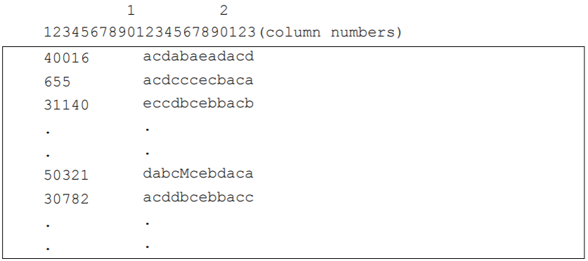
Extract from the Data File `ex1_dat.txt` [^2.11L45]

Figure 2.79: Extract from the Data File ex1_dat.txt ³¹

In this sample analysis, the generalised model for dichotomously-scored items will be fitted to the data. Traditional item analysis statistics are generated.

2.11.2 Syntax

ex10.cqc is the command file used in this tutorial to analyse the data; the file is shown in the code box below. Each line of commands in ex10.cqc is detailed in the list underneath the command file.

ex10.cqc:

Datafile ex1_dat.txt;
Format id 1-5 responses 12-23;
Labels << ex1_lab.txt;
set lconstraints=cases;
Key acddbcebbacc ! 1;
Model item!scoresfree;
Estimate;
Show  !filetype=xlsx  >> Results/ex10_shw.xlsx;
Itanal!filetype=xlsx  >> Results/ex10_itn.xlsx;
Plot icc! filesave=yes >> Results/ex10_;
Plot mcc! legend=yes,filesave=yes >> Results/ex10_;
plot icc! gins=all,raw=no,overlay=yes,filesave=yes >> Results/ex10_;

Line 1
The datafile statement indicates the name and location of the data file. Any file name that is valid for the operating system you are using can be used here.
Line 2
The format statement describes the layout of the data in the file ex1_dat.txt. This format statement indicates that a field that will be called id is located in columns 1 through 5 and that the responses to the items are in columns 12 through 23 of the data file. Every format statement must give the location of the responses. In fact, the explicit variable responses must appear in the format statement or ACER ConQuest will not run. In this particular sample analysis, the responses are those made by the students to the multiple choice items; and, by default, item will be the implicit variable name that is used to indicate these responses. The levels of the item variable (that is, item 1, item 2 and so on) are implicitly identified through their location within the set of responses (called the response block) in the format statement; thus, in this sample analysis, the data for item 1 is located in column 12, the data for item 2 is in column 13, and so on.
Line 3
The labels statement indicates that a set of labels for the variables (in this case, the items) is to be read from the file ex1_lab.txt. An extract of ex1_lab.txt is shown in Figure 2.80. (This file must be text only; if you create or edit the file with a word processor, make sure that you save it using the text only option.) The first line of the file contains the special symbol ===> (a string of three equals signs and a greater than sign) followed by one or more spaces and then the name of the variable to which the labels are to apply (in this case, item). The subsequent lines contain two pieces of information separated by one or more spaces. The first value on each line is the level of the variable (in this case, item) to which a label is to be attached, and the second value is the label. If a label includes spaces, then it must be enclosed in double quotation marks (” “). In this sample analysis, the label for item 1 is BSMMA01, the label for item 2 is BSMMA02, and so on.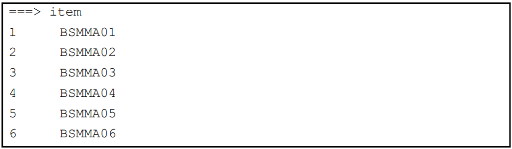

Figure 2.80: Contents of the Label File ex1_lab.txt
Line 4
The set statement specifies new values for a range of ACER ConQuest system variables. In this case, the use of the lconstraints argument is setting the identification constraints to cases. Therefore, the constraints will be set through the population model by forcing the means of the latent variables to be set to zero and allowing all item parameters (difficulty and discrimination) to be free. The use of cases as the identification constraint is required when estimating a 2PL.
Line 5
The key statement identifies the correct response for each of the multiple choice test items. In this case, the correct answer for item 1 is a, the correct answer for item 2 is c, the correct answer for item 3 is d, and so on. The length of the argument in the key statement is 12 characters, which is the length of the response block given in the format statement. If a key statement is provided, ACER ConQuest will recode the data so that any response a to item 1 will be recoded to the value given in the key statement option (in this case, 1). All other responses to item 1 will be recoded to the value of the key_default (in this case, 0). Similarly, any response c to item 2 will be recoded to 1, while all other responses to item 2 will be recoded to 0; and so on.
Line 6
The model statement must be provided before any traditional or item response analyses can be undertaken. In this example, the argument for the model statement is the name of the variable that identifies the response data that are to be analysed (in this case, item). The option scoresfree indicates that a score is to be estimated for each scoring category. In this case the data are dichotomously coded, so the resulting model is the 2PL model.
Line 7
The estimate statement initiates the estimation of the item response model.
Line 8
The show statement produces a sequence of tables that summarise the results of fitting the item response model. The option filetype sets the format of the results file, in this case an Excel file. The redirection symbol (>>) is used so that the results will be written to the file ex10_shw.xlsx in your current directory.
Line 9
The itanal statement produces a display of the results of a traditional item analysis. As with the show statement, the results are redirected to a file (in this case, ex10_itn.xlsx).
Line 10
The plot icc statement will produce 12 item characteristic curve plots, one for each item. The plots will compare the modelled item characteristic curves with the empirical item characteristic curves. The option filesave indicates that the resulting plot will be saved into a file in your working directory. The redirection symbol (>>) is used so that the plots will be written to png files named ex10_. The name of the file will be completed with ‘item X’ where the X represents the number of the item (e.g.ex10_item7). Note that the plot command is not available in the console version of ACER ConQuest.
Line 11
The plot mcc statement will produce 12 category characteristic curve plots, one for each item. The plots will compare the modelled item characteristic curves with the empirical item characteristic curves (for correct answers) and will also show the behaviour of the distractors. As with the plot icc statement, the results are redirected to a file (in this case, ex10_). Note that this command is not available in the console version of ACER ConQuest.
Line 12
The plot icc statement will produce 12 item characteristic curve plots, one for each item. The option gins=all indicates that one plot is provided for each listed generalised item. The use of the raw=no option prevents the display of the raw data in the plot. The overlay=yes option allows the requested plots to be shown in a single window. As with the previous plot statements, the resulting plots are saved to png files in the working directory.

2.11.3 Running the two-parameter model

To run this sample analysis, start the GUI version. Open the file ex10.cqc and choose Run\(\rightarrow\)Run All. ACER ConQuest will begin executing the statements that are in the cqc file; and as they are executed they will be echoed in the Output Window. When it reaches the estimation command ACER ConQuest will begin fitting the two-parameter model to the data. After the estimation is completed, the two statements that produce Excel files output (show and itanal) will be processed. The show statement will produce an Excel file (ex10_shw.xlsx) with nine tabs summarising the results of fitting the item response model. The itanal statement will produce an Excel file (ex10_itn.xlsx) with one tab showing items statistics. In the case of the GUI version, the plot statements will produce 25 plots altogether. 12 plots will contain the item characteristic curve by score category for each of the items in the data. 12 plots will contain the item characteristic curve by response category for each of the items in the data. The last plot statement will produce one plot with the ICC by score category for all items.

2.11.4 Results of fitting the two parameter model

As mentioned above, the show file will contain nine tabs. The first tab in the ex10_shw.xlsx file shows a summary of the estimation. An extract is shown in Figure 2.81. The table indicates the data set that set that was analysed and provides summary information about the model fitted (e.g.the number of parameters estimated, the number of iterations that the estimation took, the reason for the estimation termination).

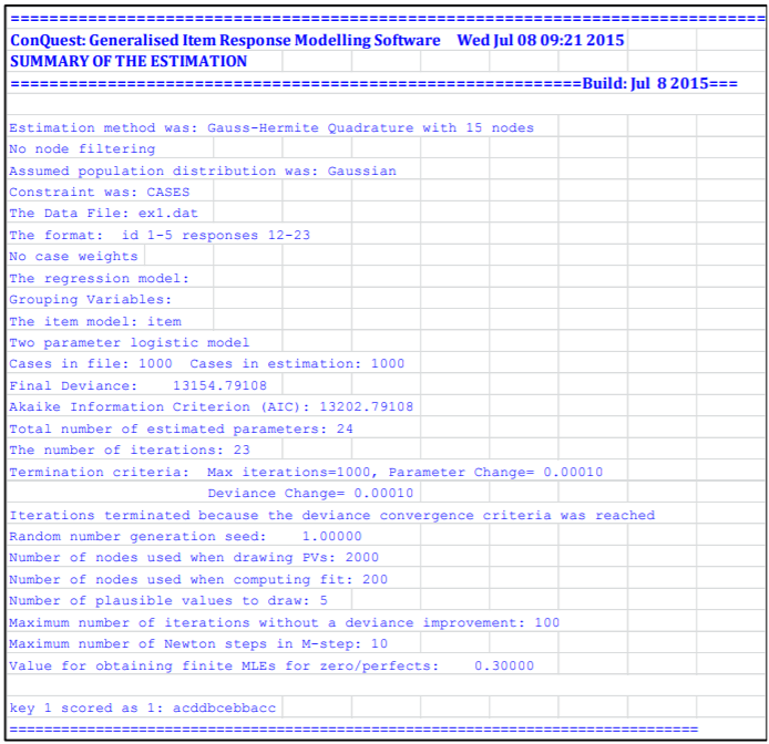
Figure 2.81: Summary of estimation Table

The second tab in the ex10_shw.xlsx Excel file gives the parameter difficulty estimates for each of the items along with their standard errors and some diagnostics tests of fit (Figure 2.82 ³²). The difficulty parameter estimates the “delta” values in equation (3) of Note 6: Score Estimation and Generalised Partial Credit Models. The last column in the table (2PL scaled estimate) shows the two-parameter scaled estimate of the item. Each value in this column is the delta value divided by the estimate of the score and is a common alternative expression of item difficulty for 2PL models. At the bottom of the table an item separation reliability and chi-squared test of parameter equality are reported.

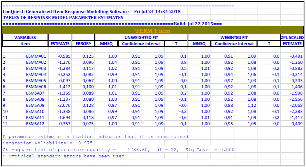
Figure 2.82: Item Parameter Estimates

The sixth and seventh tabs provide the item map of the item difficulty parameters (not shown here). The first of these maps provides an item difficulty plot according to the estimate displayed in the 2PL scaled estimate column in Figure 2.82. The second map is based on the unscaled estimate (estimate column in Figure 2.82).

For the purpose of this Tutorial, the tab of interest in the ex10_shw.xlsx Excel file is the scores tab. Here, the item discrimination parameters are presented (Figure 2.83). The score column displays the different score assigned to the correct response in each item (discrimination parameter). The error associated to the estimate is also presented.

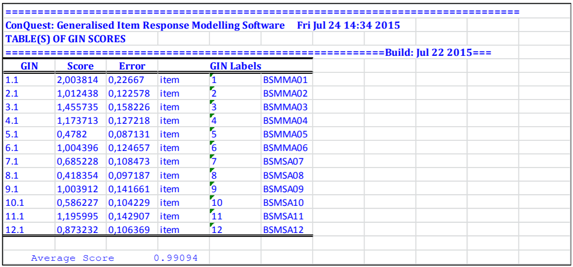
Figure 2.83: Score estimates for each item

The item analysis is shown on the ex10_itn.xlsx output file. The itanal output includes a table showing classical difficulty, discrimination, and point-biserial statistics for each item. Figure 2.84 shows the results for items 2 and 3. The 2PL discrimination estimate for each is shown in the score column. Summary results, including coefficient alpha for the test as a whole, are printed at the end of the spreadsheet.

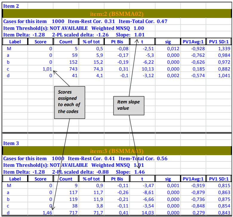
Figure 2.84: Item Analysis Results

Figure 2.85 shows plots that were produced by the plot icc and the plot mcc command for items 1 and item 5. In the left panel, the ICC plot shows a comparison of the empirical item characteristic curve (the broken line, which is based directly upon the observed data) with the modelled item characteristic curve (the smooth line).

The right panel shows a matching plot produced by the plot mcc command. In addition to showing the modelled curve and the matching empirical curve, this plot shows the characteristics of the incorrect responses — the distractors. In particular it shows the proportion of students in each of a sequence of ten ability groupings³³ that responded with each of the possible responses.

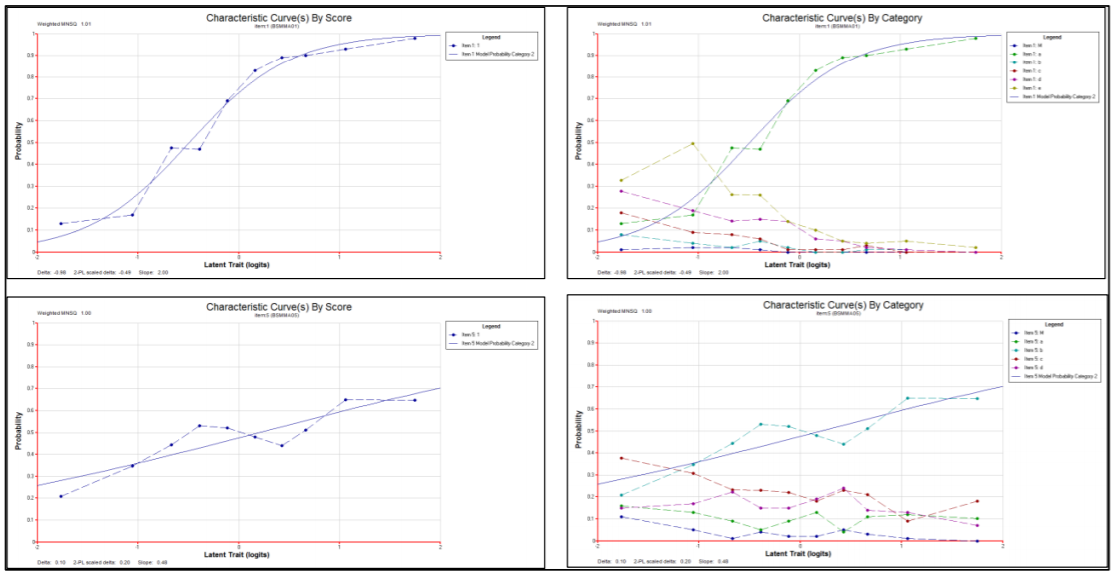
Figure 2.85: Plots for item 1 and item 5

The second plot icc command of the ex10.cqc file produces the plot shown in Figure 2.86. Here all ICCs are plotted in the same window, which allows the graphical comparison of the different discrimination capabilities of each item.

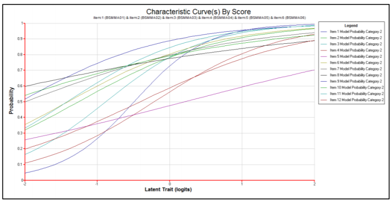
Figure 2.86: Item Characteristic Curve plot for all items in the data set

2.11.5 Summary

This tutorial shows how ACER ConQuest can be used to analyse a multiple-choice test with the 2PL model. Some key points covered in this tutorial are:

the need to set lconstraints to cases when estimation of discrimination parameters is required.
the model statement allows the estimation of different slopes (discrimination) for each item through the scoresfree option.
the itanal statement provides information about the discrimination estimate for each item.
the plot statement allows the graphical comparison of the discrimination power of each item.

2.12 Modelling Polytomous Items with the Generalised Partial Credit and Bock Nominal Response Models

As discussed in Note 6: Score Estimation and Generalised Partial Credit Models, ACER ConQuest can estimate scoring parameters for a wide range of models with polytomous data where item responses are categorical values, including multidimensional forms of the two-parameter family of models such as the multidimensional generalised partial credit models (Muraki, 1992). In addition, ACER ConQuest can also estimate scoring parameters for models with polytomous data where item responses are in the form of nominal categories, such as Bock’s nominal response model (Bock, 1972). In this tutorial, the use of ACER ConQuest to fit the generalised partial credit and Bock nominal response models is illustrated through two sets of sample analyses. Both analyses use the same cognitive items: in the first the generalised partial credit model is fitted to the data; and in the second, the Bock nominal response model is fitted.

The data for this tutorial are the responses of 515 students to a test of science concepts related to the Earth and space previously used in the Tutorial Modelling Polytomously Scored Items with the Rating Scale and Partial Credit Models.

The data have been entered into the file ex2a_dat.txt, using one line per student. A unique identification code has been entered in columns 2 through 7, and the students’ response to each of the items has been recorded in columns 10 through 17. In this data, the upper-case alphabetic characters A, B, C, D, E, F, W, and X have been used to indicate the different kinds of responses that students gave to these items. The code Z has been used to indicate data that cannot be analysed. For each item, these codes are scored (or, more correctly, mapped onto performance levels) to indicate the level of quality of the response. For example, in the case of the first item (the item in column 10), the response coded A is regarded as the best kind of response and is assigned to level 2, responses B and C are assigned to level 1, and responses W and X are assigned to level 0. An extract of the file ex2a_dat.txt is shown in Figure 2.87.

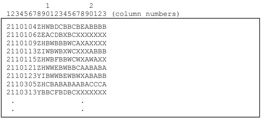
Figure 2.87: Extract from the Data File ex2a_dat.txt

2.12.1 a) Fitting the Generalised Partial Credit Model

2.12.1.1 Required files

The files used in this sample analysis are:

filename	content
ex11a.cqc	The command statements.
ex2a_dat.txt	The data.
ex2a_lab.txt	The variable labels for the items on the partial credit test.
ex11a_shw.txt	The results of the generalised partial credit analysis.
ex11a_itn.txt	The results of the traditional item analyses.

(The last two files are created when the command file is executed.)

2.12.1.2 Syntax

ex11a.cqc is the command file used to fit the Generalised Partial Credit Model in this tutorial. It is shown in the code box below, and each line of the command file is explained in the list underneath the code.

ex11a.cqc:

Title Generalised Partial Credit Model: What happened last night;
data ex2a_dat.txt;
format name 2-7 responses 10-17;
labels << ex2a_lab.txt;
codes 3,2,1,0;
set lconstraints=cases;
recode (A,B,C,W,X) (2,1,1,0,0)            !items(1);
recode (A,B,C,W,X) (3,2,1,0,0)            !items(2);
recode (A,B,C,D,E,F,W,X) (3,2,2,1,1,0,0,0)!items(3);
recode (A,B,C,W,X) (2,1,0,0,0)            !items(4);
recode (A,B,C,D,E,W,X) (3,2,1,1,1,0,0)    !items(5);
recode (A,B,W,X) (2,1,0,0)                !items(6);
recode (A,B,C,W,X) (3,2,1,0,0)            !items(7);
recode (A,B,C,D,W,X) (3,2,1,1,0,0)        !items(8);
model item + item*step!scoresfree;
estimate;
show !estimates=latent >> Results/ex11a_shw.txt;
itanal >> Results/ex11a_itn.txt;
plot expected >> Results/ex11a_expected_;
plot mcc >> Results/ex11a_mcc_;

Line 1
Gives a title for this analysis. The text supplied after the command title will appear on the top of any printed ACER ConQuest output. If a title is not provided, the default, ConQuest: Generalised Item Response Modelling Software, will be used.
Line 2
Indicates the name and location of the data file. Any name that is valid for the operating system you are using can be used here.
Line 3
The format statement describes the layout of the data in the file ex2a_dat.txt. This format indicates that a field called name is located in columns 2 through 7 and that the responses to the items are in columns 10 through 17 (the response block) of the data file.
Line 4
A set of labels for the items are to be read from the file ex2a_lab.txt. If you take a look at these labels, you will notice that they are quite long. ACER ConQuest labels can be of any length, but most ACER ConQuest printouts are limited to displaying many fewer characters than this. For example, the tables of parameter estimates produced by the show statement will display only the first 11 characters of the labels.
Line 5
The codes statement is used to restrict the list of codes that ACER ConQuest will consider valid. This meant that any character in the response block defined by the format statement—except a blank or a period (.) character (the default missing-response codes) — was considered valid data. In this sample analysis, the valid codes have been limited to the digits 0, 1, 2 and 3; any other codes for the items will be treated as missing response data. It is important to note that the codes statement refers to the codes after the application of any recodes.
Line 6
The lconstraints=cases argument of the set command is used to have the mean of each latent dimension set to zero, rather than the mean of the item parameters on each dimension set to zero (e.g., lconstraints=items). All item parameters are still estimated, but the mean of each of the latent dimensions is set to zero.
Lines 7-14
The eight recode statements are used to collapse the alphabetic response categories into a smaller set of categories that are labelled with the digits 0, 1, 2 and 3. Each of these recode statements consists of three components. The first component is a list of codes contained within parentheses. These are codes that will be found in the data file ex2a_dat.txt, and these are called the from codes. The second component is also a list of codes contained within parentheses, these codes are called the to codes. The length of the to codes list must match the length of the from codes list. When ACER ConQuest finds a response that matches a from code, it will change (or recode) it to the corresponding to code. The third component (the option of the recode command) gives the levels of the variables for which the recode is to be applied. Line 11, for example, says that, for item 6, A is to be recoded to 2, B is to be recoded to 1, and W and X are both to be recoded to 0. Any codes in the response block of the data file that do not match a code in the from list will be left untouched. In these data, the Z codes are left untouched; and since Z is not listed as a valid code, all such data will be treated as missing-response data. When ACER ConQuest models these data, the number of response categories that will be assumed for each item will be determined from the number of distinct codes for that item. Item 1 has three distinct codes (2, 1 and 0), so three categories will be modelled; item 2 has four distinct codes (3, 2, 1 and 0), so four categories will be modelled.
Line 15
The model statement for these data contains two terms (item and item*step) and will result in the estimation of two sets of parameters. The term item results in the estimation of a set of item difficulty parameters, and the term item*step results in a set of item step-parameters that are allowed to vary across the items. The option scoresfree results in the estimation of an additional set of item scores that are allowed to vary across the items. This is the generalised partial credit model.

In the section The Structure of ACER ConQuest Design Matrices, there is a description of how the terms in the model statement specify different versions of the item response model. In addition, Note 6: Score Estimation and Generalised Partial Credit Models describes how ACER ConQuest estimates the score parameters in models such as the generalised partial credit model.
Line 16
The estimate statement is used to initiate the estimation of the item response model.
Line 17
The show statement produces a display of the item response model parameter estimates and saves them to the file ex11a_shw.txt. The option estimates=latent requests that the displays include an illustration of the latent ability distribution.
Line 18
The itanal statement produces a display of the results of a traditional item analysis. As with the show statement, the results have been redirected to a file (in this case, ex11a_itn.txt).
Lines 19-20
The plot statements produce two displays for each item in the test. The first requested plot is a comparison of the observed and the modelled expected score curve, while the second is a comparison of the observed and modelled item characteristics curves by category.

2.12.1.3 Running the Generalised Partial Credit sample analysis

To run this sample analysis, start the GUI version. Open the file ex11a.cqc and choose Run\(\rightarrow\)Run All.

ACER ConQuest will begin executing the statements that are in the file ex11a.cqc; and as they are executed, they will be echoed on the screen. When ACER ConQuest reaches the estimate statement, it will begin fitting the generalised partial credit model to the data, and as it does so it will report on the progress of the estimation.

After the estimation is complete, the two statements that produce output (show and itanal) will be processed. The show statement will produce seven separate tables. All of these tables will be in the file ex11a_shw.txt. The contents of the first table were discussed in the Tutorial A Dichotomously Scored Multiple Choice Test, and the contents of the second one in the Tutorial Modelling Polytomously Scored Items with the Rating Scale and Partial Credit Models. The third table (not shown here) gives the estimates of the population parameters. In this case, the mean of the latent ability distribution was constrained to 0.000, and the variance of that distribution constrained to 1.000.

The fifth table was also discussed in the Tutorial Modelling Polytomously Scored Items with the Rating Scale and Partial Credit Models, and is a map of the parameter estimates and latent ability distribution. However, with the exception of predicted probability maps, item maps are not applicable for models with estimated scores. The sixth table, which contains information related to the item score estimates produced by the scoresfree argument in the model statement, is shown in Figure 2.88. The score parameter estimates are reported for each category of each generalised item, although for the generalised partial credit model ACER ConQuest only estimates a single parameter for each item, shown in the final (seventh) table of the show file, discussed later.

For the first item, two score estimates have been reported, corresponding to the codes (1, 2) that this item can take in the data (code 0 will always be scored as zero). For the second item, three score estimates have been reported, corresponding to the codes (1, 2, 3) that this item can take in the data.

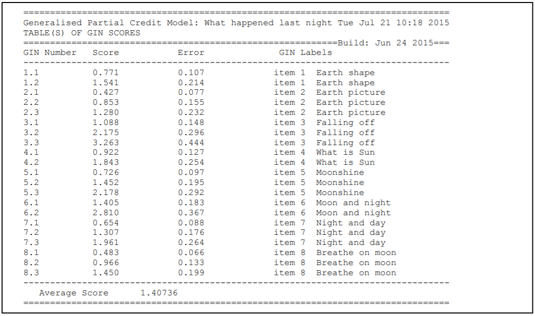
Figure 2.88: Item Score Parameters Estimated by the Generalised Partial Credit Model

Figure 2.89 shows the seventh table, which displays the Tau parameter estimates for each item and associated standard errors. This estimate is applied to each category of each generalised item to estimate the score parameter estimates that were produced in the previous table. If you compare the sixth and seventh tables, you will notice that the first score estimate for each item in the sixth table is the same as the Tau estimate for that item in the seventh table. The second score estimate (corresponding to category 2) is then double the Tau value, the third score estimate (corresponding to category 3) is triple the Tau value, and so on. Regardless of how many categories each item has, only a single Tau parameter is estimated by the model. This Tau parameter is an estimate of each item’s discrimination.

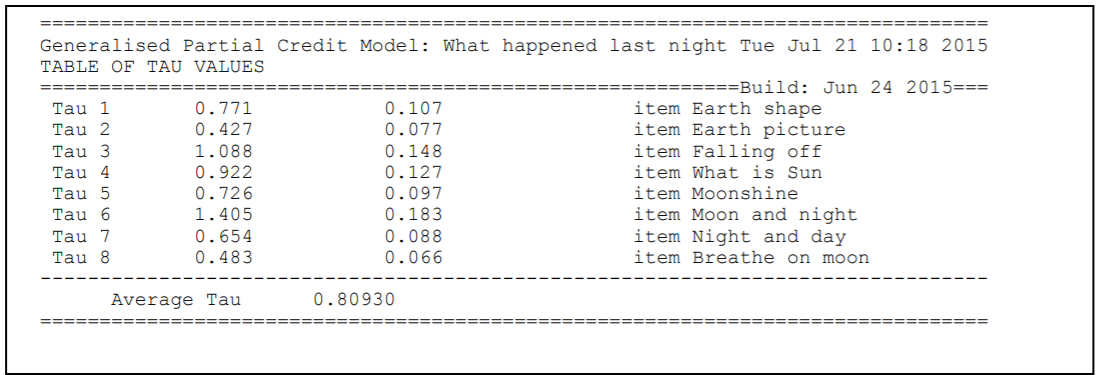
Figure 2.89: Tau Parameters Estimated by the Generalised Partial Credit Model

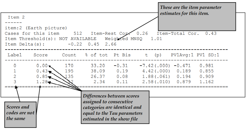
Figure 2.90: Extract of Item Analysis Printout for a Polytomously Scored Item Estimated with the Generalised Partial Credit Model

The itanal command in line 18 produces a file (ex11a_itn.txt) that contains traditional item statistics (Figure 2.90). In this example a key statement was not used and the items use partial credit scoring. As a consequence the itanal results are provided at the level of scores, rather than response categories. As you can see in the output, the scores reported are those estimated by the model, not the codes that the response categories are assigned in the data. For the generalised partial credit model, the difference between the scores assigned to consecutive response categories is the same for all categories that item has, and corresponds to the Tau value estimated for that item in the show file. In this case, you can see in Figure 2.89 that the Tau value for item 2 is 0.427, which is equal to the difference between the scores assigned to consecutive categories shown in Figure 2.90.

The plot commands in line 19 and 20 produce the graphs shown in Figure 2.91. For illustrative purposes only plots for item 1 and 2 are shown. The second item showed poor fit to the scaling model — in this case the generalised partial credit model.

The second item’s Tau value of 0.427 indicates that this item is less discriminating than the first item (Tau=0.771). The comparison of the observed and modelled expected score curves (the plots appearing on the left of the figure) is the best illustration of this lower discrimination. Notice how for the second item’s plot the observed curve is a little flatter than the modelled curve. This will often be the case when the item discrimination is low.

The plots appearing on the right of the figure show the item characteristic curves, both modelled and empirical. There is one pair of curves for each possible score on the item. Note that for item 2 the disparity between the observed and modelled curves for category 2 is the largest. The second part of this tutorial will demonstrate how ACER ConQuest can estimate scores for each category of each item in the model, to determine how well each category score fits the scaling model.

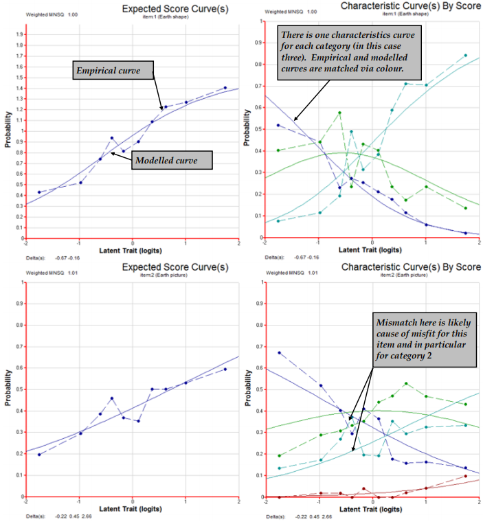
Figure 2.91: Plots for Items 1 and 2

2.12.2 b) Bock’s Nominal Response Model

In the second sample analysis of this tutorial, the Bock nominal response model is fitted to the same data used in the previous analysis, to illustrate the differences between the two models.

2.12.2.1 Required files

The files that we use are:

filename	content
ex11b.cqc	The command statements.
ex2a_dat.txt	The data.
ex2a_lab.txt	The variable labels for the items on the test.
ex11b_shw.txt	The results of the nominal response analysis.
ex11b_itn.txt	The results of the traditional item analyses.

(The last two files are created when the command file is executed.)

2.12.2.2 Syntax

The command file for fitting the Bock nominal response model to the data is ex11b.cqc; it is shown in the code box below. In the list following the code box each line of commands is explained in detail.

ex11b.cqc:

Title Bock Nominal Response Analysis: What happened last night;
datafile ex2a_dat.txt;
format name 2-7 responses 10-17;
labels << ex2a_lab.txt;
codes 3,2,1,0;
set lconstraints=cases;
recode (A,B,C,W,X) (2,1,1,0,0)            !items(1);
recode (A,B,C,W,X) (3,2,1,0,0)            !items(2);
recode (A,B,C,D,E,F,W,X) (3,2,2,1,1,0,0,0)!items(3);
recode (A,B,C,W,X) (2,1,0,0,0)            !items(4);
recode (A,B,C,D,E,W,X) (3,2,1,1,1,0,0)    !items(5);
recode (A,B,W,X) (2,1,0,0)                !items(6);
recode (A,B,C,W,X) (3,2,1,0,0)            !items(7);
recode (A,B,C,D,W,X) (3,2,1,1,0,0)        !items(8);
model item + item*step!bock;
estimate;
show !estimates=latent >> Results/ex11b_shw.txt;
itanal >> Results/ex11b_itn.txt;
plot expected >> Results/ex11b_expected_;
plot mcc >> Results/ex11b_mcc_;

Line 1 For this analysis, we are using the title Bock Nominal Response Analysis: What happened last night.
Lines 2-14 The commands in these lines are exactly the same as for the generalised partial credit model analysis (see above).
Line 15 The model statement for these data is exactly the same as for the generalised partial credit model analysis. The option bock results in the estimation of an additional set of item category scores that are allowed to vary across each of the categories of each of the items. This is the Bock nominal response model.
Lines 16-20 The commands in these lines are exactly the same as for the generalised partial credit model analysis (see above), however the names of the show and traditional item (itanal) analysis files have been changed to ex11b_shw.txt and ex11b_itn.txt, respectively.

2.12.2.3 Running the Bock Nominal Response Sample Analysis

To run this sample analysis, start the GUI version. Open the file ex11b.cqc and choose Run\(\rightarrow\)Run All.

ACER ConQuest will begin executing the statements that are in the file ex11b.cqc; and as they are executed, they will be echoed on the screen. When ACER ConQuest reaches the estimate statement, it will begin fitting the Bock nominal response model to the data, and as it does so it will report on the progress of the estimation.

After the estimation is complete, the two statements that produce output (show and itanal) will be processed. The show statement will again produce seven separate tables. All of these tables will be in the file ex11b_shw.txt, and are the same as those described in the generalised partial credit model (see above).

The important difference between this model and the generalised partial credit model is illustrated in the sixth and seventh tables in the show file. The sixth table, contains information related to the item score estimates produced by the bock option in the model statement, is shown in Figure 2.92. The score parameter estimates are reported for each category of each item, and in this case ACER ConQuest estimates a single parameter for each category of each item (rather than a single parameter for each item, as was the case for the generalised partial credit model).

As with the generalised partial credit model, two score estimates have been reported for the first item, corresponding to the codes (1, 2) that this item can take in the data (code 0 will always be scored as zero). For the second item, three score estimates have been reported, corresponding to the codes (1, 2, 3) that this item can take in the data.

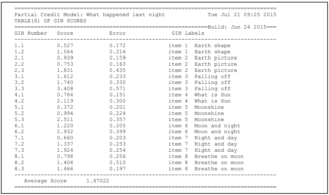
Figure 2.92: Item Score Parameters Estimated by Bock’s Nominal Response Model

Figure 2.93 shows the seventh table, which displays the Tau parameter estimates for each item and associated standard errors, as it did for the generalised partial credit model. However, you will notice that there are more values in this table than there was for the generalised partial credit model. This is because ACER ConQuest is estimating score parameters for each category of each item individually. Consequently, there is a one-to-one correspondence between the values in this table and those that were reported in the previous table. These Tau parameters provide an estimate of each item category’s discrimination.

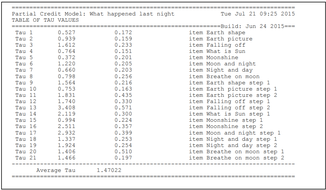
Figure 2.93: Tau Parameters Estimated by Bock’s Nominal Response Model

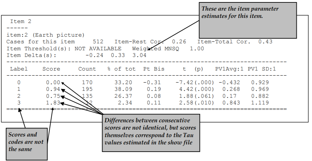
Figure 2.94: Extract of Item Analysis Printout for a Polytomous Item Estimated with Bock’s Nominal Response Model

The itanal command in line 18 produces a file (ex11b_itn.txt) that contains traditional item statistics (Figure 2.94). In this example, as with the generalised partial credit example, a key statement was not used and the items use partial credit scoring. As a consequence the itanal results are provided at the level of scores, rather than response categories. As you can see in the output, the scores reported are those estimated by the model, not the codes that the response categories are assigned in the data. These scores correspond to the Tau values estimated in the show file in Figure 2.93, as well as the score values in Figure 2.92, as the Tau and score parameters are identical in the Bock nominal response model.

As you can see in both the show file and the traditional item statistics, the category scores estimated by ACER ConQuest can differ quite substantially to the codes that were manually allocated to the data values. In an example with ordinal response data such as this, the order of the category scores estimated by ACER ConQuest should match the order of the codes that were in the data (so that a code of 2 gets a higher score than a code of 1). You can see in this example that this is not the case for item 2. The scores estimated by ACER ConQuest for codes 1, 2 and 3 are 0.939, 0.753, and 1.831 respectively. As the score estimated for code 2 is less than that estimated for code 1, this points to a problem in the coding of the original data.

The plot commands in lines 19 and 20 produce the graphs shown in Figure 2.95. For illustrative purposes only plots for item 1 and 2 are shown. These graphs show a similar picture to what was shown in the generalised partial credit example. The disparity between the observed and modelled item characteristic curves for category 2 of item 2 that was noted in the generalised partial credit example is still observed here, and supported by the discrepancy between the scores estimated for this item in the show file and traditional item statistics.

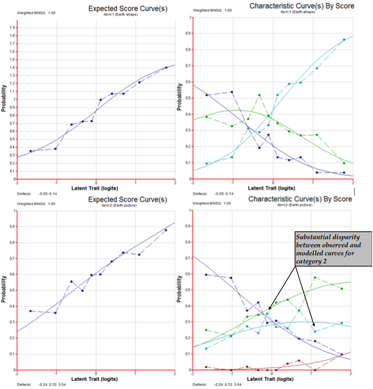
Figure 2.95: Plots for Items 1 and 2

2.12.3 Summary

In this tutorial, ACER ConQuest has been used to fit the generalised partial credit and Bock nominal response models. Some key points covered were:

The scoresfree option in the model statement can be used to estimate a single parameter for each item in a given dataset which is used to determine scores that each item category receives (generalised partial credit model).
The bock option in the model statement can be used to estimate a score for each category of each item in a given dataset (bock nominal response model).
The score parameters estimated by ACER ConQuest can be used to determine item fit (generalised partial credit model) as well as item category fit (bock nominal response model).

2.13 The use of Matrix Variables in examining DIF

The purpose of this tutorial is to illustrate the use of matrix variables. Matrix variables are internal (matrix valued) objects that can be created by various ACER ConQuest procedures, or read into ACER ConQuest and then manipulated. For example the estimate command can create matrix variables that store the outcomes of the estimation³⁴. Matrix variables can be manipulated, saved or plotted.

In this Tutorial we show how subsets of the data can be analysed to evaluate differential item functioning. In this case we analyse differences between male and female students. We show how the results can be stored as matrix variables and how those matrices can be manipulated and plotted.

2.13.1 Required files

The files used in this sample analysis are:

filename	content
ex12.cqc	The command statements.
ex5_dat.txt	The data.
ex6_lab.txt	The variable labels for the items on the multiple choice test.

The ex5_dat.txt file contains achievement for 6800 students. Each line in the file represents one tested student. The first 19 columns of the data set contain identification and demographic information for each student. Columns 20 to 176 contain student responses to multiple-choice, and short and extended answer items. For the multiple-choice items, the codes 1, 2, 3, 4 and 5 are used to indicate the response alternatives to the items. For the short answer and extended response items, the codes 0, 1, 2 and 3 are used to indicate the student’s score on the item. If an item was not presented to a student, the code . (dot/period) is used; if the student failed to attempt an item and that item is part of a block of non-attempts at the end of a test, then the code R is used. For all other non-attempts, the code M is used. More information about the ex5_dat.txt file can be found in the Tutorial Unidimensional Latent Regression. An extract from the data file is shown in Figure 2.96.

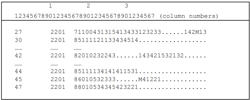
Extract from the Data File `ex5_dat.txt` [^2.13L42]

Figure 2.96: Extract from the Data File ex5_dat.txt ³⁵

In this example, only data from columns 16 to 25 are used. Column 16 contains the code for the booklet that each student responded; the range is 1 to 8. Column 17 contains the code 0 for male students and 1 for female students. Column 18 contains the code 0 for lower grade (first year of secondary school) students and 1 for upper grade (second year of secondary school) students. Column 19 contains the product of columns 17 and 18, that is, it contains 1 for upper grade female students and 0 otherwise. Columns 20 to 25 contain the student responses to the first six items in the database. These six items are dichotomously scored.

In this sample analysis, the simple logistic model will be fitted to the data to analyse differences in item difficulty between boys and girls using graphic displays.

2.13.2 Syntax

Below we show the contents of the command file used in this analysis, ex12.cqc, followed by a description of each line of syntax.

ex12.cqc:

datafile ex5_dat.txt;
title TIMSS Mathematics--First Six Items;
set lconstraints=cases;
format book 16 gender 17 level 18 gbyl 19 responses 20-25;
labels << ex6_lab.txt;
key 134423 ! 1;
model item;
keepcases 0! gender;
estimate!matrixout=male;
reset;

datafile ex5_dat.txt;
title TIMSS Mathematics--First Six Items;
set lconstraints=cases;
format book 16 gender 17 level 18 gbyl 19 responses 20-25;
labels << ex6_lab.txt;
key 134423 ! 1;
model item;
keepcases 1! gender;
estimate!matrixout=female;


/* create data to plot an identity line */
compute itemparams=male_itemparams->female_itemparams;
let identityx=matrix(2:1);
let identityy=matrix(2:1);
compute identityx[1,1]=min(itemparams);
compute identityy[1,1]=min(itemparams);
compute identityx[2,1]=max(itemparams);
compute identityy[2,1]=max(itemparams);

/* plot the relationship */
scatter identityx,identityy!join=yes,seriesname=identity;
scatter male_itemparams,female_itemparams!overlay=yes,
                                          legend=yes,
                                          xmax=1,
                                          xmin=-2,
                                          ymax=1,
                                          ymin=-2,
                                          seriesname=male vs female,
                                          title=Comparison of Item Parameter Estimates,
                                          subtitle=Male versus Female;


/* centre the item parameter estimates for both groups on zero
 and compute differences */
compute male_itemparams=male_itemparams-sum(male_itemparams)/rows(male_itemparams);
compute female_itemparams=female_itemparams-sum(female_itemparams)/rows(female_itemparams);
compute difference=male_itemparams-female_itemparams;

/* extract the standard errors from the error covariance matrix */
let var_male=matrix(6:1);
let var_female=matrix(6:1);
for (i in 1:6)
{
    compute var_male[i,1]=male_estimatecovariances[i,i];
    compute var_female[i,1]=female_estimatecovariances[i,i];
};

/* create data to plot upper and low 95% CI on Wald test */
let upx=matrix(2:1);
let upy=matrix(2:1);
let downx=matrix(2:1);
let downy=matrix(2:1);
compute upx[1,1]=1;
compute upy[1,1]=1.96;
compute upx[2,1]=rows(difference);
compute upy[2,1]=1.96;
compute downx[1,1]=1;
compute downy[1,1]=-1.96;
compute downx[2,1]=rows(difference);
compute downy[2,1]=-1.96;
compute item=counter(rows(difference));

/* calculate SE of difference and Wald test */
compute se_difference=sqrt(var_male+var_female);
compute wald=difference//se_difference;

/* plot standard differences */
scatter upx,upy!join=yes,seriesname=95 PCT CI Upper;
scatter downx,downy!join=yes,overlay=yes,seriesname=95 PCT CI Lower;
scatter item,wald!join=yes,
                  overlay=yes,
                  legend=yes,
                  seriesname=Wald Values,
                  title=Wald Tests by Item,
                  subtitle=Male versus Female;

Line 1
The datafile statement indicates the name and location of the data file. Any file name that is valid for the operating system you are using can be used here.
Line 2
The title statement specifies the title that is to appear at the top of any printed ACER ConQuest output.
Line 3
The set statement specifies new values for a range of ACER ConQuest system variables. In this case, the use of the lconstraints argument is setting the identification constraints to cases. Therefore, the constraints will be set through the population model by forcing the means of the latent variables to be set to zero and allowing all item parameters (difficulty and discrimination) to be free.
Line 4
The format statement describes the layout of the data in the file ex5_dat.txt. This format statement indicates the name of the fields and their location in the data file. For example, the field called book is located in column 16 and the field called gender is located in column 17. The responses to the six items used in this tutorial are in columns 20 through 25 of the data file.
Line 5
The labels statement indicates that a set of labels for the variables (in this case, the items) is to be read from the file ex6_lab.txt. An extract of ex6_lab.txt is shown in Figure 2.97. (This file must be text only; if you create or edit the file with a word processor, make sure that you save it using the text only option.)

The first line of the file contains the special symbol ===> (a string of three equals signs and a greater than sign) followed by one or more spaces and then the name of the variable to which the labels are to apply (in this case, item). The subsequent lines contain two pieces of information separated by one or more spaces. The first value on each line is the level of the variable (in this case, item) to which a label is to be attached, and the second value is the label. If a label includes spaces, then it must be enclosed in double quotation marks (" "). In this sample analysis, the label for item 1 is BSMMA01, the label for item 2 is BSMMA02, and so on.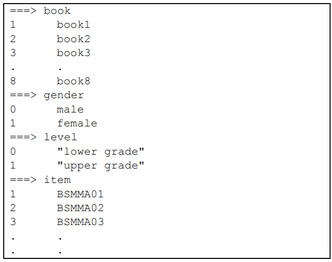

Figure 2.97: Contents of the Label File ex6_lab.txt
Line 6
The key statement identifies the correct response for each of the multiple choice test items. In this case, the correct answer for item 1 is 1, the correct answer for item 2 is 3, the correct answer for item 3 is 4, and so on. The length of the argument in the key statement is 6 characters, which is the length of the response block given in the format statement.

If a key statement is provided, ACER ConQuest will recode the data so that any response 1 to item 1 will be recoded to the value given in the key statement option (in this case, 1). All other responses to item 1 will be recoded to the value of the key_default (in this case, 0). Similarly, any response 3 to item 2 will be recoded to 1, while all other responses to item 2 will be recoded to 0; and so on.
Line 7
The model statement must be provided before any traditional or item response analyses can be undertaken. In this example, the argument for the model statement is the name of the variable that identifies the response data that are to be analysed (in this case, item). By omitting the option statement we are fitting a rasch model where scores for each item are fixed.
Line 8
The keepcases statement specifies a list of values for explicit variables that if not matched will be dropped from the analysis. The keepcases command can use two possible types of matching:
1. EXACT matching occurs when a code in the data is compared to a keep code value using an exact string match. A code will be treated as a keep value if the code string matches the keep string exactly, including leading or trailing blank characters. Values placed in double quotes are matched with this approach.
2. The alternative is TRIM matching, which first trims leading and trailing spaces from both the keep string and the code string and then compares the results. Values not in quotes are matched with this approach. To ensure TRIM matching of a blank or a period character, the words blank and dot are used. The list of codes should be followed by the name of the explicit variables where these codes are to be found. If there is more than one variable, they should be comma separated.
In this case, we are keeping the code 0 for the variable gender, therefore modelling only males’ responses. All cases with value 1 in this variable will be excluded from the analysis. By using the keepcases command we estimate separate item parameters for these two groups of students, producing separate matrix variables for males and females. We then use these matrix variables to evaluate DIF.
Line 9
The estimate statement initiates the estimation of the item response model. The matrixout option indicates that a set of matrices with prefix male_ will be created to hold the results. This matrix will be stored in the temporary workspace. Any existing matrices with matching names will be overwritten without warning.

The Matrices produced by estimate depend upon the options chosen. The list of matrices is found in Figure 2.98 and their content is described in the section Matrix Objects Created by Analysis Commands. You can see these matrices using the print command or using the workspace menu in the GUI mode.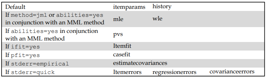

Figure 2.98: Matrices created by the estimate command
Line 10
The reset command resets ACER ConQuest system values to their default values, except for tokens and variables. The command is used here to erase the effects of previously issued commands.
Lines 12-20
This set of commands is exactly the same to that mentioned above, with the exception of the last two (estimate and keepcases). In this part of the ex12.cqc file, we are modelling responses for females. Therefore, the keepcases statement instructs ACER ConQuest to keep in the analysis only those cases where the value of the variable gender equals 1. A set of matrices named with the prefix female_ will hold the results of the estimated model (estimate statement).

In Lines 23-42 of ex12.cqc, data is extracted from the two matrices created above with the estimate statement. The data is used to create an identity line and then plotted to show differences in item difficulty for males and females.

Line 24
The compute command takes the male_itemparams and the female_itemparams object from the matrices created with the estimate statements. By using the -> operator these two matrices are concatenated in a new matrix named itemparams. The new matrix contains six rows and two columns. The rows, one for each item, contain the estimated item location parameters (difficulty) and the columns correspond to student gender, male and female. For a list of compute command operators and functions see section 4.8.
Lines 25-26
The two let statements define two empty matrices, identityx and identityy, each with two rows and one column. These matrices allow us to draw the identity line in the scatter plot created below.
Lines 27-30
The compute statements fill the two newly created matrices with the minimum and maximum values observed in the matrix itemparams. Both matrices are filled with the same values.
Line 33
The scatter statement produces a scatter plot of two variables. In this case, identityx and identityy. The join option indicates that the two points are to be joined by a line; in this case, the identity line. The seriesname option defines the text to be used as a series name. The plot is displayed as a separate window in the screen and is shown in Figure 2.99.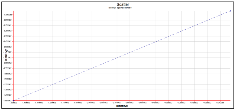

Figure 2.99: Scatter plot for the identity line
Lines 34-42
The second scatter statement produces a scatter plot of the item parameters for males and females (Figure 2.100). The overlay option allows the resulting plot to be overlayed on the existing active plot. In this case, results will be overlayed with the identity line shown in Figure 2.99. The option legend indicates that legend is displayed. The xmax, xmin, ymax and ymin options set the maximum and minimum values for the horizontal and vertical axes of the plot, respectively and overwrite the values on the previous plot. The seriesname option specifies the text to be used as series name. The title and subtitle options specify the text to be used as title and subtitle of the plot.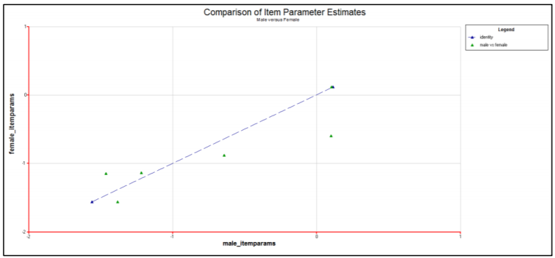

Figure 2.100: Scatter plot of item parameters for males and females

The set of statements in Lines 45-87 of ex12.cqc centres the item parameters for both groups on zero and computes the difference between them for each item. With these results and the standard errors from the covariance matrix, a scatter plot is produced to display the Wald test of differences between the two groups (Engle, 1984). The plot also includes 95% confident levels for the Wald test.

Lines 47-49
The compute statement centres the item parameters (e.g.male_itemparams) by subtracting the mean of the item difficulties (e.g.sum(male_itemparams)/rows(male_itemparams)) to each item. A matrix with the centred values of item parameters is computed for each group. The difference of item difficulties between the two groups is also computed and stored in a new matrix named difference.
Lines 52-53
The let statements create two 6 by 1 empty matrices — one for each group.
Lines 54-58
The for statement fills the above created matrices with the values of the estimate error variance for each item. These values are found in the diagonal of the estimates error variance-covariance matrix that is produced in the estimate statement (rows 9 and 18 in the command file ex12.cqc.).
Lines 61-64
The let statements create four 2 by 1 empty matrices, upx, upy, downx, and downy so we can plot the confidence interval lines in the plot.
Lines 65-72
The compute statements fill the matrices with the following values.
- The element in the first row and column (i.e. [1,1]) of the matrices upx and downx with the number 1.
- The element in the second row and first column (i.e., [2,1]) of the matrices upx and downx with the number of rows of the difference matrix (i.e., 6).
- The first and second rows of the matrices upy and downy with the number 1.96 and -1.96, respectively.
Line 73
The compute statement creates a variable named item. The function counter creates a matrix with the same number of rows as the difference matrix (i.e., 6) and 1 column, filled with integers running from 1 to 6. This serves for producing the horizontal axis in the scatter plot described in the last scatter statement in ex12.cqc.
Lines 76-77
The compute statements define two 6 by 1 matrices: se_difference and wald. The row values in the first of these matrices correspond to the square root (sqrt) of the sum of variances for each item between groups (var_male+var_female). By using the // operator, the values in the Wald matrix are computed as the division of each element in the difference matrix by the matching element in the se_difference matrix. The Wald test can be used to test for standard differences in item parameters between two groups, males and females in this case.
Line 80
The scatter statement produces a scatter plot of the upx and upy matrix variables. The plot is displayed on a new window. The values 1 and 6 in the horizontal axis and the value 1.96 in the vertical axis. The option join specifies a line that joins the points in the horizontal axis. The seriesname option defines the text to be used as series name.
Line 81
The scatter statement produces a scatter plot of the downx and downy matrix variables. The values 1 and 6 in the horizontal axis and the value -1.96 in the vertical axis. The option join specifies a line that joins the points in the horizontal axis. The overlay option indicates that the resulting plot is overlayed with the active plot produced by the previous scatter statement. The seriesname option defines the text to be used as series name.
Lines 82-87
The last scatter statement produces a scatter plot of the item and wald matrix variables (Figure 2.101). The item matrix, with values from 1 to 6 is displayed in the horizontal axis. And the wald matrix in the vertical axis. The plot is overlayed with the active plot produced by the two previous scatter statements by using the option overlay. The legend is set to be displayed by using the option legend. The name of the new series added to the plot is set with the seriesname option. The title and subtitle are also specified with the corresponding options.

To avoid having a large number of decimal places in the values of the Wald test you have two options. One is to specify the upper and lower values of the vertical axis using the ymax and ymin options in the scatter statement. Another is to manipulate the graph via the PlotQuest window menus. The second approach is the one we used in Figure 2.101.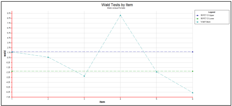

Figure 2.101: Wald test for standardised differences in item estimates between males and females

2.13.3 Running the Analysis

To run this sample analysis, start the GUI version. Open the file ex12.cqc and choose Run\(\rightarrow\)Run All.

ACER ConQuest will begin executing the statements that are in the file ex12.cqc; and as they are executed they will be echoed in the Output Window. When it reaches the estimate command ACER ConQuest will begin fitting the two-parameter model to the data.

After the estimation is completed, the scatter statements will produce two plots that will be displayed in new windows. The first of these plots contains a comparison of the item parameter estimates for males and females, and also displays the identity line. The second plot contains the Wald test of standardized differences in item parameters for these two groups, along with the 95% confidence intervals.

As mentioned above, the first plot produced by the ex12.cqc file contains a comparison of the item estimates for males and females, along with the identity line. The plot is shown in Figure 2.100. According to the plot, there seems to be some variation in item difficulties for these two groups of students. An item where difference is more noticeable and thus of particular interest is item four (the one in the low right corner). Other items showing some degree of variability between the two groups are items three and six (the two on the left bottom corner).

The plot in Figure 2.101 allows us to determine whether the differences observed in the previous plot are statistically significant. In fact, items three, four and six are those where the Wald values fall considerable outside of the confidence interval, showing presence of DIF between the males and females. Wald values for items one and two are within the confidence interval, which indicates that although these items have different difficulty parameters for males and females, the difference is not statistically significant. Wald value of item five is just outside of the confidence interval; a close inspection of the item to investigate DIF is recommended.

2.13.4 Summary

This tutorial shows how ACER ConQuest matrix variables can be used to evaluate Differential Item Functioning (DIF) between two groups. Some key points covered in this tutorial are:

the use of the keepcases command allows the estimation of item parameters separately for different groups.
the use of the matrixout option in the estimate statement allows holding the results for each group in separate matrix variables.
the use of operators and functions associated to the compute statement provide the opportunity to manipulate matrix variables created through the estimate command and compute new variables.
the scatter statement allows the graphical comparison of the item parameters for different groups of students.

2.14 Modelling Pairwise Comparisons using the Bradley-Terry-Luce (BTL) Model

2.14.1 Background³⁶

ACER ConQuest can be used to fit a logistic pairwise comparison model, also known as the Bradley-Terry-Luce (BTL) model (Bradley & Terry, 1952; Luce, 2005). Discussed in Note 2: Pairwise Comparisons, pairwise comparison is an approach to estimate a single parameter based on paired comparisons. The paired comparisons may be subjective (e.g., subjective rankings of two objects) or objective (e.g., winner in a paired game). The pairwise comparison approach is useful because there are situations where it is easier to make judgements between two objects than it is to rank all objects at once. It is easier to discriminate between two objects than to differentiate among a large set of objects and place them on an interval scale.

There are also situations where direct ranking may not be feasible (for example if there are a large number of objects to rank). In the example used in this tutorial, a sports tournament, estimating team strengths using the BTL model requires data on each team’s performance against a set of opponents with each game treated as a pairwise comparison having a dichotomous outcome (win or lose).

In the original Bradley-Terry (1952) model, the probability of success (or higher rank) of an object in the pair is given as:

\[\begin{equation} P_{ij}=\frac{\delta_i}{\delta_i+\delta_j} \tag{2.1} \end{equation}\]

where \(P_{ij}\) denotes the probability that object \(i\) is ranked higher than object \(j\) (or that \(i\) wins over \(j\)), and \(\delta\) is the scale location parameter for objects \(i\) and \(j\). It can be shown that for any pair \((i, j)\) if one wins the other loses, as shown in the derivation below (Glickman, 1999):

\[\begin{equation} \begin{split} P_{ij}+P_{ji} & = \frac{\delta_i}{\delta_i+\delta_j}+\frac{\delta_j}{\delta_j+\delta_i} \\ & = \frac{\delta_i+\delta_j}{\delta_i+\delta_j} \\ & = 1 \end{split} \tag{2.2} \end{equation}\]

Reparametrising the model in terms of the fixed pair \(i,j\) where \(x_{ij}=1\) if \(i\) is ranked higher and \(x_{ij}=0\) if \(i\) is ranked lower, we have the BTL model as presented in Note 2:

\[\begin{equation} P(X_{ij} = 1;\delta_i, \delta_j)=\frac{exp(x_{ij}\delta_i-(1-x_{ij})\delta_j)}{1+exp(\delta_i-\delta_j)} \tag{2.3} \end{equation}\]

2.14.2 Required files

The data for the sample analysis are the game results of 16 teams over 2,123 games. The data is formatted such that the outcome (1=win, 0=loss) refers to the team designated as object \(i\), and entered as the first of the pair.

The files used in this sample analysis are:

filename	content
ex13.cqc	The command statements.
ex13_dat.txt	The data.
ex13_ObjectLocations.png	The Wright Map plot displaying the object locations graphically.
ex13_shw.txt	The results of the pairwise comparison, showing the parameter estimates and their standard errors.
ex13_res.csv	The residuals (difference between observed and predicted (probability i wins) result).

(The last three files are created when the command file is executed.)

The data have been entered into the file ex13_dat.txt, using one line per game. The data is in fixed format, the teams designated as object \(i\) have been recorded in columns 1 through 13, while teams designated as object \(j\) have been recorded in columns 14 through 26. The value for the outcome is indicated in column 38. An extract of the file ex13_dat.txt is shown in Figure 2.102.

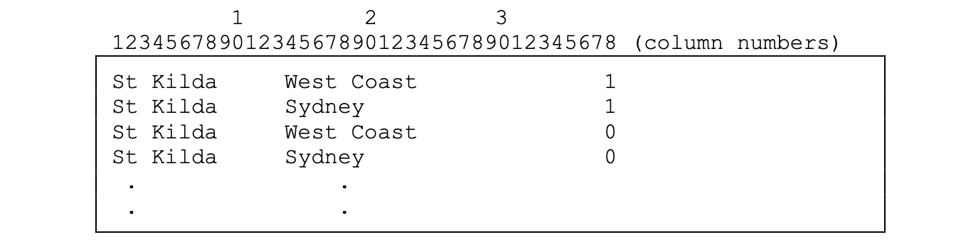
Figure 2.102: Extract from the Data File ex2a.dat

2.14.3 Syntax

The contents of the command file for this sample analysis (ex13.cqc) are shown in the code box below. Each of the command statements is explained in the list underneath the command file.

ex13.cqc:

title  Pairwise Analysis of Australian Football League;
data ex13_dat.txt;
format team1 1-13 team2 14-26 responses 38;
model team1-team2 ! type = pairwise;
estimate! stderr=quick;
plot wrightmap ! order = value, estimate = wle, rout = Results/wm >> Results/ex13_;
show >> Results/ex13_shw.txt;
show residuals !filetype=csv >> Results/ex13_res.csv;
show parameters! filetype=xlsx >> Results/ex13_prm.xlsx;

Line 1
gives a title for this analysis. The text supplied after the command title will appear on the top of any printed ACER ConQuest output. If a title is not provided, the default, ConQuest: Generalised Item Response Modelling Software, will be used.
Line 2
indicates the name and location of the data file. Any name that is valid for the operating system you are using can be used here.
Line 3
The format statement describes the layout of the data in the file ex13_dat.txt. This format indicates that a field called team1 is located in columns 1 through 13 and that team2 is located in columns 14 through 26; the outcomes of each pairwise comparison are in column 38 of the data file.
Line 4
The model statement for the pairwise analysis, showing which two objects are being compared (team1 and team2).
Line 5
The estimate statement is used to initiate the estimation of the item response model. The estimate statement requires that quick standard errors (stderr=quick) are used for pairwise comparisons.
Line 6
The plot statement will display the item locations graphically on a Wright Map. The order=value option is available for Wright Maps and displays the objects ordered by their scale location parameters (in this case, the team strength). The Wright Map only displays weighted likelihood parameter estimates (estimates=wle) in pairwise comparisons.
Line 7
The show statement produces a display of the item response model parameter estimates and saves them to the file ex13_shw.txt. The show file output is different in pairwise comparisons compared to the usual ACER ConQuest 1PL and 2PL model outputs. The show file only provides a list of the parameter estimates and their standard errors. Population parameters and traditional item statistics are not applicable with the pairwise model.
Line 8
The show residuals statement requests residuals for each fixed pair-outcome combination. These results are written to the file ex13_res.csv and are only available for weighted likelihood estimates.

2.14.4 Running the Analysis

To run this sample analysis, start the GUI version. Open the file ex13.cqc and choose Run\(\rightarrow\)Run All. ACER ConQuest will begin executing the statements that are in the file ex13.cqc; and as they are executed, they will be echoed on the screen. When ACER ConQuest reaches the estimate statement, it will begin fitting the BTL model to the data, and as it does so it will report on the progress of the estimation.

After the estimation is complete, the outputs will be produced. The first show statement will produce a summary output and one table that shows the parameter estimates of each team and the standard errors of these parameter estimates. This output is in the file ex13_shw.txt (by default, ACER ConQuest will add an appropriate file extension to all outputs). The parameter estimates are in logits and placed on an interval scale, thereby allowing for evaluating the relative differences between the teams using a uniform unit of measurement. The location parameters are constrained to a mean of zero.

Figure 2.103 shows the location parameter estimates for each of the 16 teams. Results show that Geelong is the strongest team while Richmond is the weakest.

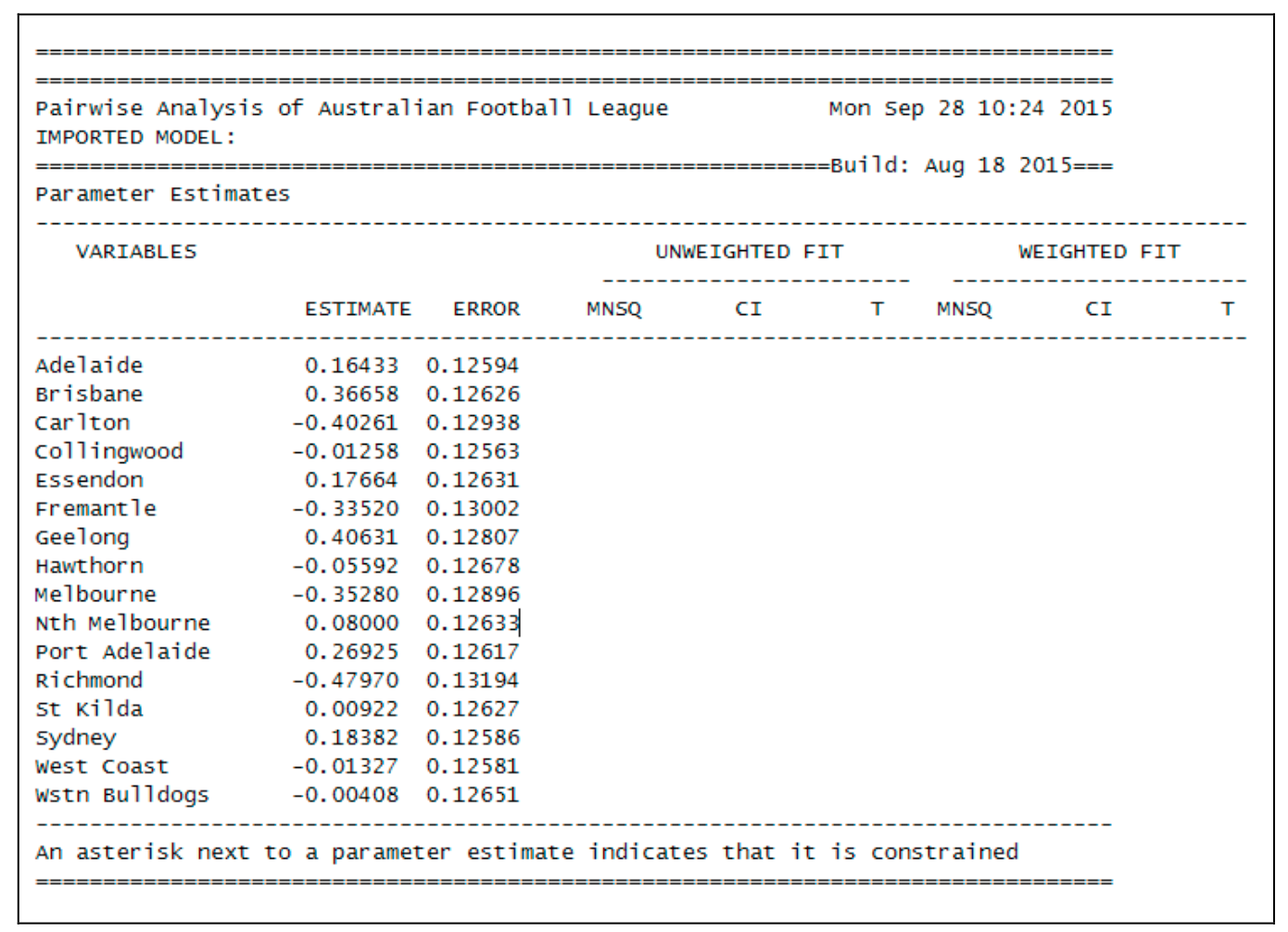
Figure 2.103: Table of item parameter esitmates

The show residuals statement produces an Excel file ex13_res.csv. Figure 2.104 shows the contents of the residuals table in ex13_res.csv. These are the residuals for each game and can be interpreted as prediction errors for each game based on the estimated team strengths.

Similar to the interpretation of residuals in regression, where \(r_{ij} = Y_{ij}-P_{ij}\). That is, the residual \(r_{ij}\) for a particular game for a particular pair \(i,j\) is the difference between the observed outcome \(Y_{ij}\) (1 if \(i\) actually won, 0 if i lost) and the predicted outcome \(P_{ij}\) (the probability that \(i\) wins over \(j\)).

This residuals table can be summarised (filtered or sorted) by team1, team2, and magnitude of residual value to assess the predictive power of the model and check unusually high prediction errors for some teams.

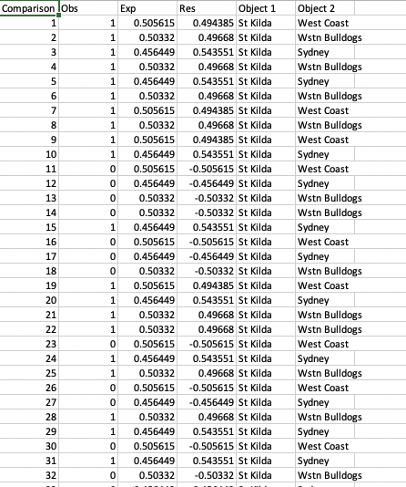
Figure 2.104: Extract of table of residuals for each paired comparison

The plot command produce the plot shown in Figure 2.105, which shows all the teams plotted against the location parameter estimate axis (i.e., team strength). The order=value option arranges the teams based on their parameter value for easier comparison and ranking. The plot also presents visually which teams have similar strengths as well as the relative differences in strength among the teams.

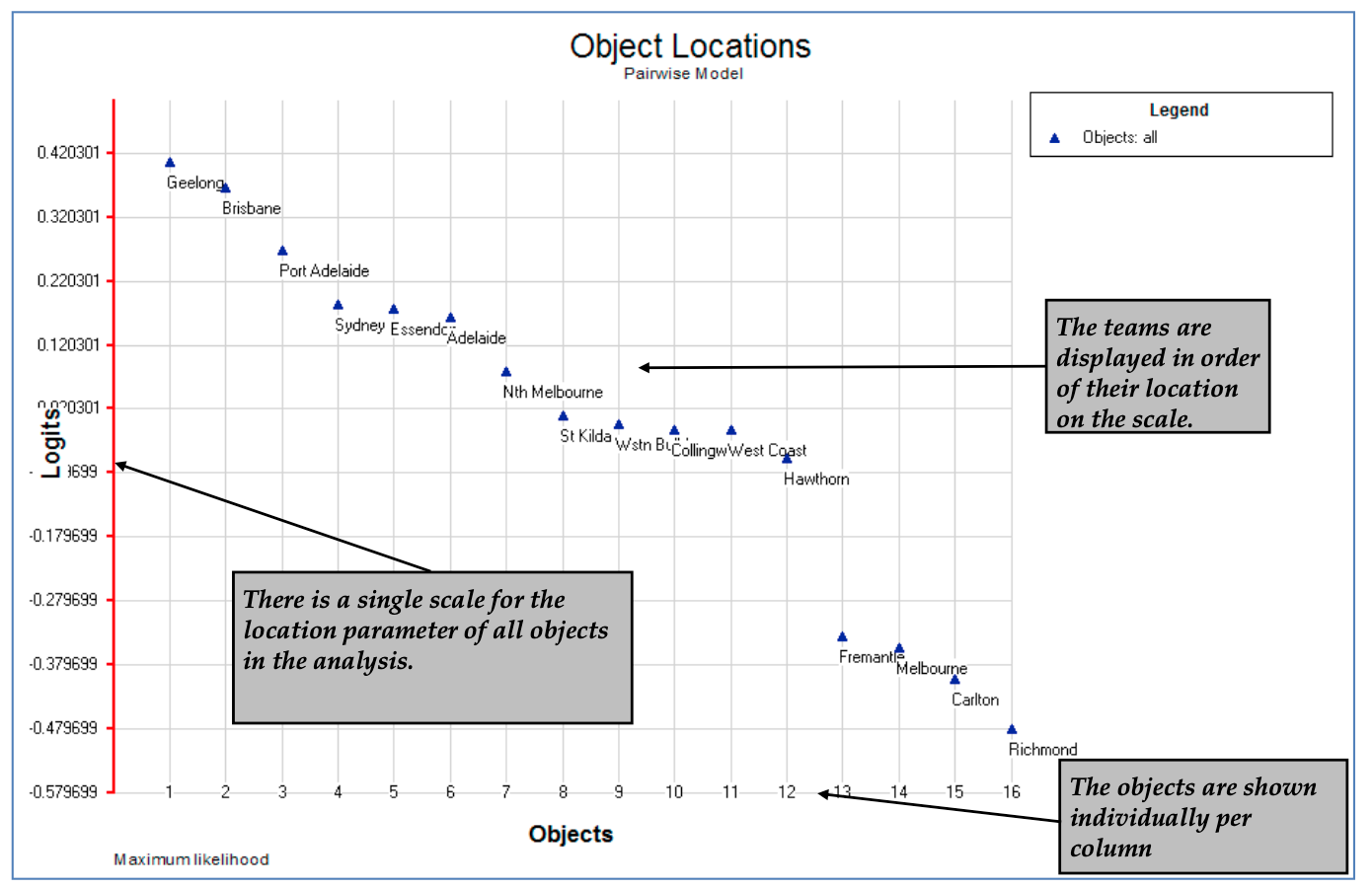
Figure 2.105: Wright Map of location parameter estimates of all teams

2.14.5 Summary

In this tutorial, ACER ConQuest has been used to fit the BTL model for a pairwise comparison analysis. Some key points covered were:

The pairwise option in the model statement can be used to estimate a BTL model given dataset which contains paired comparisons and dichotomous outcomes for each comparison.
The object location parameters estimated by ACER ConQuest can be used for ordinal comparison data to determine the location of an object on an interval scale.
The plots visually show the relative locations of the objects and can be used to visually represent the rankings.

2.15 Fitting IRTree response models

2.15.1 Background

This tutorial demonstrates how to fit IRTree models with ACER ConQuest. We will fit one of the models that was applied to intelligence test data by De Boeck & Partchev (2012). These researchers applied a variety of IRTree models to investigate the relationship between so-called fast and slow intelligence, with responses to items partitioned into fast and slow responses respectively. Multiple latent variables were specified to model the speed and accuracy processes.

It is worth noting that IRTree models can also be implemented to investigate and model response processes from a single set of item responses, without the need for auxiliary timing or telemetry data. Prominent examples include modelling response styles for Likert-type questionnaire items, and modelling missing data mechanisms in educational assessments (Jeon & De Boeck, 2015).

In this tutorial we apply an IRTree model to data from a reading comprehension assessment targeted at approximately Grade 3 level. While this is a distinct construct from the intelligence tests just mentioned, reading comprehension is itself complex, and responding to multiple-choice reading comprehension questions can involve a multitude of mental processes. Therefore we were open to the possibility that response speed could be a proxy for the utilisation of different strategies and mental processes within items and within persons. We can use IRTrees to investigate whether differences in item and person parameters are observed for differentially speeded responses. At the same time we can also investigate the relationships between the latent trait pertaining to speed and the latent traits pertaining to ‘fast’ and ‘slow’ reading comprehension abilities. For more detail on how IRTrees can be used to investigate these substantive matters, the interested reader is referred to DiTrapani et al. (2016).

2.15.1.1 IRTree formulation

The IRTree models formulated here can be specified as multidimensional IRT models (see 2.8). We chose to specify a multidimensional Rasch (Rasch, 1960) model, consistent with the formulation in De Boeck & Partchev (2012).

One of the first steps in setting up an IRTree analysis from wide-format response files is to recode the data in a manner consistent with the conditional dependencies in the given IRTree. Responses to each individual item need to be separated into responses to multiple pseudo items that each correspond to a different node in the tree. These nodes play the role of latent variables in the multidimensional model, for which separate sets of item parameters and person parameters can be estimated.

In the case of fast and slow abilities, we first specify a latent variable node that represents the propensity to respond quickly. We use within-item median response times to separate responses into either fast or slow responses, much as De Boeck & Partchev (2012) did, in order to assign scores (1 for fast, 0 for slow) to pseudo items for this node. Then, for fast responses and slow responses in turn, we create pseudo items for the correctness of the response. A depiction of the corresponding response tree follows:

It follows that for any item where a student responds quickly: they will have a value of 1 for that item’s corresponding ‘speed’ pseudo item that loads onto the Speed Propensity node; they will have a value of either 0 or 1 for that item’s ‘fast and accurate’ pseudo item that loads onto the Fast Ability node; and, they will have a value of ‘missing’ for the corresponding ‘slow and accurate’ pseudo item that loads onto the Slow Ability node. For a student who responds slowly to an item: they will have a value of 0 for the ‘speed’ pseudo item; they will have a value of either 0 or 1 for the ‘slow and accurate’ pseudo item; and, they will have a value of ‘missing’ for the ‘fast and accurate’ pseudo item. This yields a total of four possible response categories per item from the original response time and response accuracy information. Usefully, the conditional independence specified between the nodes makes it possible to compute the probability that a given student will respond in any one of the four end-point categories, conditional on their propensity to respond quickly and their estimated fast and slow abilities.

2.15.1.2 Recoding responses

The process of constructing an appropriately structured and recoded data file from the original response and response time information is as follows.

We first read in the item responses and the item response times for the 32 reading comprehension multiple-choice questions for a sample of 2000 students.

We then create the ‘speed’ pseudo items by assigning all items’ responses to either fast or slow. This produces 32 such columns, one per item.

Next we create the two sets of accuracy-related pseudo items that are conditional on speed. This produces a further 32 columns for the fast responses and the slow responses respectively. Therefore there will be a total of 96 pseudo item columns in the data file to be analysed.

We can check whether the recoding is consistent with the implied conditional independence in the tree diagram. For item 10 in the sequence, we inspect the response category frequencies for fast and slow accuracies, conditional on response speed.

Item 10 fast pseudo item score frequencies for slow responses (top row) and fast responses (bottom row)
Response speed	0	1	NA
Slow	0	0	1000
Fast	116	884	0

Item 10 slow pseudo item score frequencies for slow responses (top row) and fast responses (bottom row)
Response speed	0	1	NA
Slow	267	733	0
Fast	0	0	1000

We can see that each of these accuracy pseudo items has half of its responses (1000) as 0 or 1 values, and half of its values as missing (‘NA’ is the default code for missing in the R program that was used to prepare the data). This is consistent with the within-item median split that was used for all ‘speed’ pseudo items. This shows that the data for this particular item have been partitioned appropriately for the estimation of the two separate latent abilities.

2.15.2 Required files

The files that we will use in this example are:

filename	content
ex15.cqc	The command lines used for the analysis.
ex15_data.csv	The pseudo item scored responses.
ex15_anch.dat	Anchor values for item parameters for the speed node.
ex15_shw.txt	Selected results from the analysis.

2.15.3 Syntax

The command syntax for an IRTree model is equivalent to that for a conventional between-item compensatory multidimensional model. The differences, as noted, relate more to the restructuring of the underlying response data.

The contents of the command file ex15.cqc are shown in the code box below, and explained line-by-line in the list that follows the figure.

2.15.3.1 Multidimensional Rasch formulation of an IRTree model

ex15.cqc:

title speed accuracy tree;
data ex15_data.csv ! filetype = csv,columnlabels = yes, responses = n_speed_01 to n_slow_32, width = 1;
codes 0 1;
score (0,1) (0,1) () () ! items(1-32);
score (0,1) () (0,1) () ! items(33-64);
score (0,1) () () (0,1) ! items(65-96);
import anchor_parameters << ex15_anch.dat;
model item;
estimate;
show ! estimates=latent  >> ex15_shw.txt;

Line 1
This is the title of the analysis.
Line 2
Indicates the name and location of the data file. Here we use a CSV file, as indicated following the filetype command. We retain column labels and we use these in conjunction with the responses command to name the range of columns (pseudo item responses) to include in the analysis.
Line 3
We use the codes statement to restrict the valid codes to 0 and 1. Importantly, we omit missing or blank values so that these are definitely treated as missing in the analysis.
Line 4-6
The model that we are fitting here is three dimensional, so the score statements contain four sets of parentheses as their arguments, one for the ‘from’ codes and three for the ‘to’ codes. The option of the first score statement gives the items to be assigned to the first dimension, the option of the second score statement gives the items to be allocated to the second dimension, and so on. Recall that we have a ‘speed’ dimension, followed by two ability dimensions, one fast and one slow. Earlier, we intentionally constructed the pseudo item response columns in blocks that corresponded to each of these latent variables. The sequential nature of these three blocks of items can be seen in parentheses after the term ! items at the end of each of the lines 4-6.
Line 7
We choose to anchor all item parameter values corresponding to the speed node to zero. This is because we have used a within-item median response time split (and we have very fine-grained timing data down to milliseconds), meaning that exactly half of the responses will be classified as fast and half will be classified as slow. Retaining the constraint that the mean of the item parameter values per dimension is zero, this implies that every item parameter in the speed dimension has the same relative location along the speed trait, which is necessarily zero. Anchoring is not strictly necessary, but it simplifies the estimation process since fewer parameters need to be estimated.
Line 8
The simple logistic model is used for each dimension.
Line 9
The model is estimated using the default settings.
Line 10
The show statement produces a sequence of tables that summarise the results of fitting the item response model.

2.15.4 Running the analysis

To run this sample analysis, start the GUI version. Open the file ex15.cqc and choose Run -> Run All.

Alternatively, you can launch the console version of ACER ConQuest, by typing the command (on Windows) ConQuestConsole.exe ex15.cqc.

For conquestr (Cloney & Adams, 2022) users, you can also call ACER ConQuest and run ex15.cqc using the command conquestr::ConQuestCall('ex15.cqc').

By inspecting the show file output (Figure 2.106), we can see what parameters were estimated and we can draw several salient conclusions about the relationship between fast and slow responses in the context of our reading comprehension assessment.

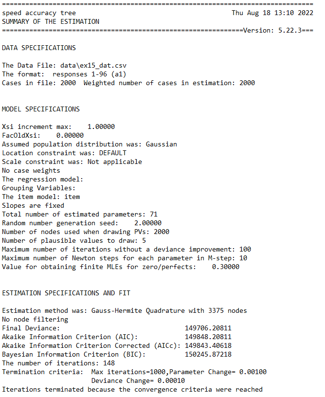
Figure 2.106: Summary of estimation information

In this analysis 71 parameters were estimated. They are:

the mean and variance of the three latent nodes that are being measured (making 6 parameters);
the covariance values between the three latent nodes (making 3 parameters); and
62 item difficulty parameters. Recall that we did not estimate any parameters for the speed dimension, and, following the usual convention of Rasch modelling, the mean of the item difficulty parameters within each dimension has been made zero, so that a total of 31 parameters is required to describe the difficulties of the 32 items.

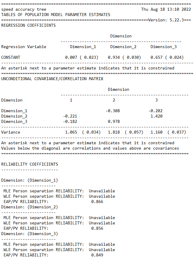
Figure 2.107: Summary of latent variable distributions

Several interesting observations can be made in relation to the covariance/correlation matrix and the variance values for each dimension:

Most notably, the latent correlation between fast and slow abilities is extremely close to one. This is reassuring, in that the test appears to measure the same underlying ability irrespective of whether students are responding quickly or slowly as defined by the within-item median split.
There is a weak negative correlation between the propensity to respond quickly and the two (ostensibly one) latent abilities. This implies that the propensity to respond quickly tends to be associated with slightly poorer performance.
The variance of the latent ability measured from fast responses is larger than that for the latent ability measured from slow responses. There appears to be more information in the fast responses than in the slow responses.

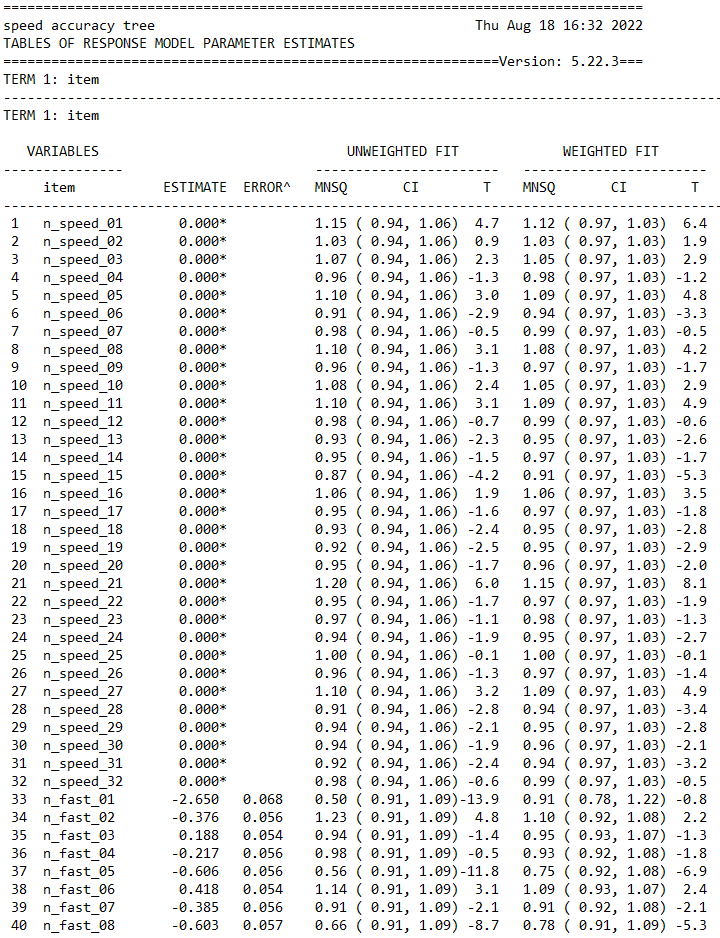
Figure 2.108: Summary of speed pseudo item parameters

We see from the first 32 item parameters that the anchoring process has been applied as intended. The parameters for all pseudo items mapped to the speed node are equal to zero. Interestingly, this dimension has a comparable level of reliability to the ability dimensions. The items also appear to fit the model reasonably well according to the fit statistics shown above.

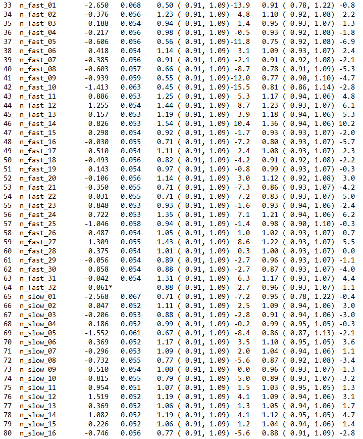
Figure 2.109: Summary of fast and slow item parameters

Looking now at the two sets of item parameters for the fast and slow ability traits, some interesting differences can be observed. While most items have similar relative difficulty between the two sets, some individual items differ more noticeably in their relative difficulties when they are responded to quickly as opposed to slowly. For example, the fifth item in the sequence (which appears at lines 37 and 69) differs more than is the case for most items, with the difference being almost one logit (though note that these scales are not directly comparable). This item appears to be easier when it is responded to more slowly. An obvious follow up activity is to qualitatively review this item in light of these findings, and to attempt to devise some hypotheses for the differential item difficulty under fast and slow responses.

2.15.5 Summary

In this section we have illustrated how ACER ConQuest can be used to fit IRTree models. Specifically, we fit a one-parameter IRTree model and interpreted various features of the output.

Some key points that were covered include:

IRTree models can be specified as multidimensional models with an appropriate restructuring and recoding of response data.
A variety of response processes can be investiagted using IRTree models.
Insights can be gained into how item parameters and latent abilities change under different processes.
Insights can be gained into how different latent abilities relating to different aspects of a response process are related to one another.
It is possible to carry out model comparisons that compare different assumptions about response processes and associated latent traits. As an example, it is possible to show that a model with the latent correlation between fast and slow abilities constrained to equal one has a marginally lower BIC than the unconstrained model shown in this tutorial. This provides some support for the claim that fast and slow abilities can be treated as equivalent for this reading comprehension test (though Log-Likelihood and AIC slightly prefer the unconstrained model, so the statistical support is slightly equivocal).

We use the notation File\(\rightarrow\)Open to indicate that the menu item Open should be chosen from the File menu.↩︎
The term ‘student’ or ‘students’ is used to indicate the object of the measurement process, that is, the entity that is being measured. This term has been chosen because most of the sample analyses are set in an educational context where the object of measurement is typically a student. The methods, however, are applicable well beyond the measurement of students.↩︎
The analysis of dichotomous tests with traditional methods is usually referred to as classical test theory.↩︎
If you wish to launch ACER ConQuest in this fashion on command-based systems, ConQuestConsole.exe must be in the directory you are working in or a path must have been set up; otherwise, you must type the entire path name.↩︎
In this case the single term was ‘item’.↩︎
Ten ability groupings is a default setting that can be altered.↩︎
The agents of measurement are the tools that are used to stimulate responses. They are typically test items or, more generally, assessment tasks.↩︎
The object of measurement is the entity that is to be measured, most commonly a student, a candidate or a research subject.↩︎
Fischer (1973) recognised that items could be described by more fundamental parameters when he proposed the linear logistic test model. Linacre (1994) extended the model to the polytomous case and recognised that the more fundamental components could be raters and such.↩︎
OP (overall performance) is a judgment of the task fulfilment, particularly in terms of appropriateness for purpose and audience, conceptual complexity, and organisation of the piece. TF (textual features) focuses on control and effective use of syntactic features, such as cohesion, subordination, and verb forms, and other linguistic features, such as spelling and punctuation.↩︎
Generalised item is the term that ACER ConQuest uses to refer to each of the unique combinations of the facets that are the agents of measurements.↩︎
ACER ConQuest can model up to 50 different facets.↩︎
For those familiar with approach and terminology of Linacre (1994), these would be considered four-faceted data, since Linacre counts the cases as a facet, whereas we count the unique variables in the model statement.↩︎
For uses of initial value files and anchor files, see sections 2.6 and 2.9.↩︎
See Estimation in Chapter 3 for further explanation of the estimation methods that are used in ACER ConQuest.↩︎
These 6800 students were randomly selected from a larger Australian TIMSS sample of over 13 000 students in their first two years of secondary schooling.↩︎
The current version of ACER ConQuest does not report standardised regression coefficients or standard errors for the regression parameter estimates. Plausible values can be generated (via show cases !estimates=plausible) and analysed to obtain estimates of standard errors and to obtain standardised regression coefficients.↩︎
The file ex5a.out contains the EAP and maximum likelihood ability estimates merged with the level variable for the 6800 students. The file contains one line per student, and the fields in the file are sequence number, level, maximum likelihood ability estimate (fourth field in Figure 2.44), EAP ability estimate when level is used as a regression variable (third field in Figure 2.45 and EAP ability estimate when no regressor is used.↩︎
The file ex5b.out contains the EAP ability estimates merged with the level variable for all 6800 students. The file contains one line per student and the fields in the file are sequence number, the level variable, EAP ability estimate when level is used as a regression variable, and EAP ability estimate when no regressor is used.↩︎
The standard deviation is around 1.1 (See section 2.6). The results reported here should not be extrapolated to the Australian TIMSS data. The significance testing done here does not take account of the design effects that exist in TIMSS due to the cluster sampling that was used, further they are based on a random selection of half of the TIMSS data set.↩︎
Although ACER ConQuest will permit the analysis of up to 30 dimensions, our simulation studies suggest that there may be moderate bias in the estimates of the latent covariance matrix for models with more than eight dimensions (Volodin & Adams, 1995).↩︎
The file ex7a.out (provided with the samples) contains the data used in computing the results shown in Figure 2.60. The fixed-format file contains eight fields in this order: mathematics raw score, science raw score, mathematics MLE, science MLE, mathematics EAP from the joint calibration, science EAP from the joint calibration, mathematics EAP from separate calibrations, and science EAP from separate calibrations.↩︎
Here we are using the KR-20 index that is reported by ACER ConQuest at the end of the printout from an itanal analysis.↩︎
See Adams et al. (1991) for how the socio-economic indicator was constructed.↩︎
The current version of ACER ConQuest does not report standardised regression coefficients or standard errors for the regression parameter estimates. Plausible values can be generated (as explained later in this section) and analysed to obtain estimates of standard errors and to obtain standardised coefficients.↩︎
Simulation studies (Volodin & Adams, 1995) suggest that 1000 to 2000 nodes may be needed for accurate estimation of the variance-covariance matrix.↩︎
The EAP values in Figures 2.70 and 2.71 are not the same, because ACER ConQuest selects a different random number generator seed each time EAP values are generated.↩︎
This would be necessary if a latent regression model were being estimated.↩︎
ACER ConQuest will attempt to build a design for within-item multidimensional models, but this design will be incorrect if lconstraints=cases is not used.↩︎
In Figure 2.79, each column of the data file is labelled so that it can be easily referred to in the text. The actual ACER ConQuest data file does not have any column labels.↩︎
Note: the tables in Figs. 2.82–2.84 show decimal commas in the parameter estimates. Different versions of Excel might render decimal marks differently (e.g., as ‘dot’).↩︎
Ten ability groupings is a default setting that can be altered.↩︎
For a list of commands that can produce matrix variables and the content of those variables see the section Matrix Objects Created by Analysis Commands.↩︎
In Figure 2.96, each column of the data file is labelled so that it can be easily referred to in the text. The actual ACER ConQuest data file does not have any column labels.↩︎
This is an updated document based on the original, authored by Alvin Vista and Ray Adams, 12 October 2015.↩︎