Chapter 4 ACER ConQuest Command Reference
This chapter contains general information about the syntax of ACER ConQuest command statements followed by an alphabetical reference of ACER ConQuest commands.
All ACER ConQuest commands can be accessed through a command line interface. In addition, the majority of commands with their options can be accessed through the graphical user interface. The graphical user interface is only available for Windows operating systems. This document describes the syntax for the command line interface and the graphical user interface accessibility of each of these commands.
4.1 Command Statement Syntax
An ACER ConQuest statement can consist of between one and five components: a command, arguments, options, an outdirection and an indirection. The general syntax of an ACER ConQuest statement is as follows:
Command Arguments ! Options >> Outdirection << Indirection;The first text in a statement must be a command.
The command can be followed by an argument with a space used as a separator.
Some commands have optional arguments; others require an argument.
An exclamation mark (!) separates arguments from options; if there is no argument,
the exclamation mark can separate a command from an option.
Where there is more than one legal option they are provided as a comma separated list of options.
The value passed into the option (on the right hand side of the equals sign) can be a
string literal or a variable. For options that take a boolean value, this can be represented as:
- the string
trueorfalse - the string
yesorno - the number
1or0 - a matrix variable, of which the first element evaluates to
1or0
The characters << or >> separate a file redirection (either an indirection or an outdirection)
from the preceding elements of the statement.
ACER ConQuest syntax has the following additional features:
- A statement must be terminated with a semi-colon (
;). A statement can continue over many lines or many statements can appear on a single line. - A statement can be 16 000 characters in length and can cover any number of lines on the screen or in a command file. No continuation character is required.
- Comments are placed between
/*and*/. They can appear anywhere in a command file, and their length is unlimited. Comments cannot be nested inside another comment. - The command language is not case sensitive.
All commands and matrix objects names are folded to lower case.
Values in files are case sensitive, eg arguments for the commands
codes,keepcasesanddropcases.
- The order in which command statements can be entered into ACER ConQuest is not fixed.
There are, however, logical constraints on the ordering.
For example,
showstatements cannot precede theestimatestatement, which in turn cannot precede themodel,formatordatafilestatements, all three of which must be provided before ACER ConQuest can analyse a data set. - Any text file that you want ACER ConQuest to read must be an UTF-8 ASCII text file.
- User-provided variable names must begin with an alphabetic character and must be made up of alphabetic characters or digits. Spaces are not allowed in variable names and some characters and names are reserved for ACER ConQuest use (see List of illegal characters and words for variable names at the end of this document).
- All commands, as well as arguments and options that consist of ACER ConQuest reserved words, can be abbreviated to their shortest unambiguous root. For example, the following are all valid:
caseweight, caseweigh, caseweig, casewei, casewe, casew,
case, cas, ca
codes, code, cod, co
converge=, converg=, conver=, conve=, conv=, con=, co=
datafile, datafil, datafi, dataf, data, dat, da, d
estimate, estimat, estima, estim, esti, est, es
export, expor, expo, exp, ex
4.1.1 Example Statements
codes 0,1,2;codes is the command, and the argument is 0,1,2.
format responses 11-20 ! rater(2),essay(5);format is the command, responses 11-20 is the argument, and rater(2) and essay(5) are the options.
show ! cases=eap >> file.out;show is the command, there is no argument, cases=eap is the option, and >> file.out is the redirection.
4.2 Tokens and the Lexical Preprocessor
4.2.1 Lexical Preprocessor
Before executing a set of commands (e.g., a syntax file) the set of commands is
passed through a lexical preprocessor.
The lexical preprocessor handles the commands let, execute, dofor, doif, enddo, else and endif.
The lexical preprocessor also resolves tokens.
4.2.2 Tokens
A token is an alphanumeric string that is set by a let command. For example:
let nitems=10;
let path=C:/mywork;
After it has been defined, a token is referenced by enclosing its name
between % characters (e.g., %path%).
When a token reference is detected in a set of commands it is replaced by the value it represents.
Tokens can be used in any context.
A token is also set for each iteration of a dofor loop.
This token is referred to as the looping variable and cannot be defined prior to the dofor loop.
The tokens version, date, platform, process, tempdir and interface are created
automatically, and are available (e.g., %date%) at any time.
The process token is a unique integer associated with the current ConQuest session.
The preprocessor will literally process tokens, and so the user should ensure they
make the distinction between literal strings and strings that should be parsed.
For example, given let x = 10-1; see the distinction between:
- a string that should be parsed:
print %x%;output:9 - a literal string:
print "%x%";output:10-1
4.2.2.1 Example Statements
let n=10;
generate ! nitems=%n%;
Assigns the string 10 to the token n, so that when the subsequent generate
command is executed, the string %n% is replaced by the string 10.
dofor x=M,F;
Plot icc ! group=gender; keep=%x%;
enddo;
Produces plots for students with gender value M and then gender value F.
x is the looping variable.
4.3 Matrix Variables
A matrix variable is a matrix value that is set through a compute command or created,
when requested, by an ACER ConQuest procedure.
The command compute can be omitted, so long as the left hand side is not a protected word.
A variable can be used in a compute command, or produced by a compute command.
A variable can also be used as input in a number of procedures.
A variable can be converted to a token, for use in the command language, by the let command.
A variable can also be directly used as a component of the command language. Only
the first element (1,1) of a matrix variable is used, for example when used as a value
for an option to a command.
A number of analysis routines can be directed to save their results as variables – typically sets of matrices. These variables can be subsequently manipulated, saved or plotted.
The matrix variable version is automatically created and is an integer expression of the ConQuest version that is running.
4.3.1 Example Statements
x=10;
set seed = x;
Assigns the value 10 to the variable x and then sets the seed to the value in
the first element of x.
Note that the command compute was legally omitted.
compute n=10;
compute m=n+2;
print m;
Assigns the value 10 to the variable n, adds 2 to n and produces m and then prints
the value of m (i.e., 12).
n=fillmatrix(2,2,0);
n[1,1]=10;
n[2,1]=-23;
n[1,2]=0.4;
n[2,2]=1;
compute m=inv(n);
print n,m;
n is created as a 2 by 2 matrix which is populated with the four values, the inverse of n is then calculated and saved as m, finally the values of n and m are printed.
estimate ! matrixout=r;
compute fit=r_itemfit[,3];
plot r_itemparams fit;
print r_estimatecovariances ! filetype=xlsx >> covariances.xlsx;
Estimation is undertaken and a set of matrices containing results is created (see estimate command).
The item parameter estimates are plotted against the unweighted mean square fit statistics and then the parameter estimate covariance matrix is saved as an excel file.
4.4 Loops and Conditional Execution
Loops and conditional execution of control code can be implemented through the use of the for, while, if, dofor and doif commands.
dofor (in association with enddo) and doif (in association with endif and else) are dealt with by the preprocessor and are typically used to loop over token values or conditionally execute code based upon tokens.
4.4.1 Example Statements
doif %x%==M;
print “Plot for Males”;
plot icc ! group=gender; keep=M;
else;
print “Plot for Females”;
plot icc ! group=gender; keep=F;
endif;
Produces plots for students with gender value M or F depending upon the value of the token %x%.
The for, while, and if commands are not dealt with by the preprocessor. They are ACER ConQuest commands that are typically used to manipulate matrix variables and their contents.
4.5 Explicit and Implicit Variables
When ACER ConQuest reads data from a file identified with the datafile command with a structure as described by the format command variables of two different types can be generated. Explicit variables are variables that are listed in a format statement. Implicit variables are variables that are associated with specific columns in the data file referred to in the format statements as responses. For a full illustration of these two classes of variables see the format command.
4.6 Using ACER ConQuest Commands
ACER ConQuest is available with both a graphical user interface (GUI) and a command line, or console, interface. The ACER ConQuest command statement syntax used by the GUI and the console versions is identical. In general, the console version runs faster than the GUI version, but the GUI version is more user friendly. GUI version and console version system files are fully compatible.
4.6.1 Entering Statements via the Console Interface
When the console version of ACER ConQuest is started, the “less than” character (<) is displayed. This is the ACER ConQuest prompt. When the ACER ConQuest prompt is displayed, any appropriate ACER ConQuest statement can be entered.
As with any command line interface, ACER ConQuest attempts to execute the statement when you press the Enter key. If you have not yet entered a semi-colon (;) to indicate the end of the statement, the ACER ConQuest prompt changes to a plus sign (+) to indicate that the statement is continuing on a new line.
On many occasions, a file containing a set of ACER ConQuest statements (i.e., an ACER ConQuest command file) will be prepared with a text editor, and you will want ACER ConQuest to run the set of statements that are in the file. If we suppose the ACER ConQuest command file is called myfile.cqc, then the statements in the file can be executed in two ways.
In the first method, start ACER ConQuest and then type, at the ACER ConQuest prompt, the statement
submit myfile.cqc;A second method, which will work when running from a command-line interpreter (cmd on Windows, or Terminal on Mac), is to provide the command file as a command line argument. You launch ACER ConQuest and provide the command file in one step using47
Windows x64:
ConQuestx64console myfile.cqc;Mac:
ConQuest myfile.cqc
With either method, after you press the Enter key, ACER ConQuest will proceed to execute each statement in the file. As statements are executed, they will be echoed on the screen. If you have requested displays of the analysis results and have not redirected them to a file, they will be displayed on the screen.
4.6.2 Entering Commands via the GUI Interface
Once you have launched the GUI interface (double-click on ConQuest4GUI.exe), you can type command statements or open a command file in the GUI input window and then select
Run\(\rightarrow\)Run All.
In addition, the GUI interface has menu selections that will build and execute ACER ConQuest command statements. Access to the commands with the GUI is described seperately for each command in the Commands section below.
4.7 Commands
The remainder of this document describes the ConQuest commands. The arguments or options that are listed below the commands are reserved words when used with that command.
4.7.1 about
Reports information about this installation of ACER ConQuest. Includes the version, build, and licencing information.
4.7.2 banddefine
Defines the upper and lower bounds, and names of achievement or proficiency bands for latent scales. The proficiency bands are displayed on kidmaps.
4.7.2.2 Options
dimension =n
n is the number for the dimension of the latent model that that band/s relate to.
The default is 1, i.e. the first dimension.
upper =n
n is the upper bound of the band in logits. The default is system missing.
lower =n
n is the lower bound of the band in logits. The default is system missing.
label =string
string is the label for the band in quotes. The default is “ ”.
4.7.2.4 Examples
Banddefine ! label = "L0 (critical)", upper = -2.133, lower = -100;
Defines a band called “L0 (critical)” for the first dimension.
Note the lower bound is set at a large negative value to ensure it encompasses all of the bottom-end of the estimated scale.
4.7.2.6 Notes
- An error will be produced if bands are requested to overlap. Bands are reported on KIDMAPS when the kidmap command is called in conjunction with the option
format=samoa. - Where there is a tie, e.g., a student score is on a band boundary (e.g., the lower bound of Level 5 is 2.1 and so is the upper bound of Level 4) the student is allocated to the lower band (e.g., in this case Level 4).
4.7.3 build
Build design matrices for current model specification without proceeding to estimation.
4.7.3.4 Example
data isa.csv!filetype=csv,
              response=response,
              pid=personid,
              keeps=itemid y4 y5 y6 y7 y8 y9 y10 gender,
              keepswidth=10;
model itemid;
regression y4 y5 y6 y7 y8 y9 y10 gender;
build;                                /* build a standard design matrix */
export amatrix!filetype=matrix>>x;    /* save design as a matrix object */
4.7.4 caseweight
Specifies an explicit variable that is to be used as a case weight.
4.7.4.4 Examples
caseweight pweight ; The explicit variable pweight contains the weight for each case.
caseweight;No case weights are used.
4.7.4.5 GUI Access
Command\(\rightarrow\)Case Weight
Select the Case Weight menu item.
The radio button allows case weighting to be toggled.
If cases are to be weighted then a variable must be selected from the candidate list of explicit variables.
4.7.4.6 Notes
- The caseweight statement stays in effect until it is replaced with another caseweight statement or until a reset statement is issued. If you have run a model with case weights and then want to remove the case weights from the model, the simplest approach is to issue a caseweight statement with no arguments.
- A variable that will be a case weight must be listed in the format as an explicit variable.
- Case weighting is applied to item response model estimation, but not to traditional or descriptive statistics.
4.7.5 categorise
Sets up a dummy code for a categorical regression variable.
4.7.5.1 Argument
var(v1:v2:…:vN) or var(n)
When var is a categorical variable and n is an integer greater than
1, then the levels of the categorical varible are asumed to be a sequence of
integers from 1 to n.
When var is a categorical variable and v1:v2:…:vN is a list of values that
give levels of the categorical variable.
In both cases, by default a set of N-1 new dichotomously coded variables are created to represent the N categories of the original variable.
If the values that represent levels of the categorical variables contains leading or trailing spaces then the values will need to be enclosed in quotes. If observed levels are omitted from the list they are treated as missing data.
When var is specified as a regression variable it will be replaced by the
N-1 variables var_1, var_2, var_(N-1).
The variables var_1, var_2, var_(N-1) cannot be accessed directly
by any command.
When matching variable levels with data, two types of matches are possible. EXACT matches occur when a record within the variable is compared to categorise level value using an exact string match including leading and trailing blank characters. The alternative is a TRIM match that first trims leading and trailing spaces from both record within the variable and the categorise level.
4.7.5.2 Options
Codingmethod
method specifies the type of dummy coding. It can be one
of dummy, or effect. The default is dummy.
The first category is used as reference category.
4.7.5.4 Examples
categorise gender(M:F);Establishes “M” as a reference category so M will be coded “0” and F will be coded “1”.
categorise time(3);Establishes “1” as a reference category compared to groups coded “2” and “3”.
categorise grade(3:4:5:6:7) ! effect;Establishes four variables to represent the five response categories for grade.
Effect coding is used and the reference category is “3”.
grade=3
corresponds to
grade_1=–1, grade_2=–1, grade_3=–1, and grade_4=–1.
grade=4
corresponds to
grade_1=1, grade_2=0, grade_3=0, and grade_4=0.
grade=5
corresponds to
grade_1=0, grade_2=1, grade 3=0, and grade_4=0.
grade=6
corresponds to
grade_1=0, grade_2=0, grade_3=1, and grade_4=0.
grade=7
corresponds to
grade_1=0, grade_2=0, grade_3=0, and grade_4=1.
Categorise size (S:M:L);Establishes two variables to represent the three response categories for
size (Small, Medium and Large).
Dummy coding is used and the reference category is “S”.
size=S
corresponds to
size_1=0; and size_2=0;
size=M
corresponds to
size_1=1; and size_2=0;
size=L
corresponds to
size_1=0; and size_2=1;
4.7.5.6 Notes
- Any levels of the variable that are omitted from the code list are treated as missing data.
- To alter the reference level change the order in which the levels are listed.
- Only one variable can be processed with a categorise command. Use multiple commands to categorise multiple variables.
- The default match is a trim match, to use exact matching enclose the drop code in quotes (““)
4.7.6 chistory
Writes the commands that have been run up to the point where this command is called.
4.7.6.3 Redirection
>>filename
Show results are written to the file named filename.
If redirection is omitted, the results are written to the output window or the console.
4.7.7 clear
Removes variables or tokens from your workspace.
4.7.7.1 Argument
A comma separated list of variables and/or tokens or one of all, tokens or variables. The default is all.
4.7.7.4 Examples
clear all;Clears all variables and tokens from your workspace.
clear x, date;Deletes the variable (or tokens) x and date from your workspace.
4.7.7.5 GUI Access
Workspace\(\rightarrow\)Tokens and Variables
Results in a dialog box. The box displays the list of available tokens and variables. The Clear All or Clear Selected buttons can be used either to clear all objects listed in the box or clear the selected objects, respectively. The action takes immediate place once the button is clicked.
4.7.8 codes
Lists the characters that are to be regarded as valid data for the responses.
4.7.8.4 Examples
codes 0,1,2,3;The valid response codes are 0, 1, 2 and 3.
codes a b c d;The valid response codes are a, b, c and d.
codes 1, 2, 3, 4, 5, " ";The valid response codes are 1, 2, 3, 4, 5, and a blank.
codes " 1", " 2", " 3", "10";Each response code takes two columns. The first three that are listed have leading spaces, which must be included.
4.7.8.5 GUI Access
Command\(\rightarrow\)Codes
The list of codes must be entered using the same syntax guidelines as described above for the codelist.
4.7.8.6 Notes
- If a blank is to be used as a valid response code or if a blank is part of a valid response code, double quotation marks (
" ") must surround the response code that includes the blank. Codelistspecifies the response codes that will be valid after any recoding has been performed by therecodestatement.- If a
codesstatement is provided, then any character found in the response block of the data file (as defined by the format statement) and not found incodelistwill be treated as missing-response data. - Any missing-response codes (as defined by the
setcommand argumentmissing) incodelistwill be ignored. In other words,missingoverrides thecodesstatement. - If a
codesstatement is not provided, then all characters found in the response block of the data file, other than those specified as missing-response codes by thesetcommand argumentmissing, will be considered valid. - The number of response categories modelled by ACER ConQuest is equal to the number of unique response codes (after recoding).
- Response categories and item scores are not the same thing.
4.7.9 colnames
overwrites the names of an ACER ConQuest matrix object.
4.7.9.2 Options
A comma separated list of new column names in order and of the same length as the matrix object passed in as an argument.
4.7.9.4 Examples
mymatrix = fillmatrix(2,2,0);
write mymatrix ! filetype = csv >> mymatrix_defaultcolumnlabels.csv;
colnames mymatrix ! column1, column2;
write mymatrix ! filetype = csv >> mymatrix_customcolumnlabels.csv;
Creates a 2x2 matrix, filled with zeros. Writes the matrix, mymatrix to the file mymatrix_defaultcolumnlabels.csv with default column labels (“col_1” and “col_2”).
Overwrites the column names of mymatrix with “column1”, “column2” and saves them to the file mymatrix_customcolumnlabels.csv. Note files are saved in the current working directory, which is printed to the screen using the command dir;
4.7.9.5 Notes
- The list of column labels must be the same length as the number of columns in the matrix.
- To find the number of columns in a matrix object, use the command print, or alternatively you can assign the value to an object:
a = cols(mymatrix);
print a
4.7.10 compute
Undertakes mathematical computations and creates an ACER ConQuest data object
to store the result.
The data object can be a real number or a matrix.
The command word compute is optional and is assumed if a command word is
omitted and the argument is a legal mathematical expression.
4.7.10.1 Argument
lvalue = expression
lvalue is one of:
- The name of a matrix that will be created when
expressionis evaluated, or - A single sub-element of an existing matrix, or
expression is a legal mathematical expression in ACER ConQuest syntax.
See Compute Command Operators and Functions.
If the matrix named, lvalue already exists, it will be overwritten
when expression is evaluated.
If the user is referencing a sub-element of the matrix named, lvalue, it must
referenced by row and column and the expression must resolve to a 1x1 matrix.
4.7.10.4 Examples
compute x=10;
x=10;
Alternatives for creating a 1-by-1 matrix with x[1,1]=10.
compute x={1,2,3,4};
x={1,2,3,4};
Either form populates a pre-existing matrix with these values.
Columns cycle fastest, so the result is x[1,1]=1, x[1,2]=2, x[2,1]=3, and x[2,2]=4.
A matrix with as many elements as given numbers must have been pre-defined via a compute command.
compute x=a+b;
x=a+b;
Alternatives for creating the matrix x as matrix sum of matrices a and b.
compute m[10,3]=5;
m[10,3]=5;
Either form sets the row=10, column=3 element of the matrix m to 5.
t1=4;Produces a 1x1 matrix named, t1, where the value t[1,1] is equal to 4.
t2=fillmatrix(2,2,0);
t2={1,2,3,4};
Produces a 2x2 matrix named, t2, filled with zeros.
Then populates the elements of t2 with the values between the braces.
Values in braces must be a comma separated list of real numbers with the same
length as the number of elements in the matrix.
Note that columns cycle fastest so that the matrix is populated row-wise.
t3=identity(2);
x=2;
y=1;
t3[1,1]=20;
t3[x,y]=10;
Produces a 2x2 identity matrix named, t3 (i.e. filled with 1 on the diagonal,
and 0 on the off-diagonal elements).
Then creates a 1x1 matrix named, x, where the value x[1,1] is equal to 2.
Then creates a 1x1 matrix named, y, where the value y[1,1] is equal to 1.
Then replaces the value t3[1,1] with the value 20.
Then replaces the value t3[2,1] (note: x and y are resolved as indices of
t3) with the value 10.
Note that the row and column references must be explicit integers or passed-in
1x1 matrices.
4.7.10.6 Notes
- The available functions and operators are listed and described in section 4.8, Compute Command Operators and Functions.
- Parentheses can be nested to 10 deep.
- To populate a matrix with a set of values that matrix must be previously
defined using the
letcommand. If the right hand side of the assignment (‘=’) is a matrix or mathematical expression, then the output matrix need not be defined in advance. - Sub matrices can be extracted from matrices by
appending [
rowstart:rowend,colstart:colend] to the name of a matrix variable. If all rows are requiredrowstartandrowendcan be omitted. If all columns are requiredcolstartandcolendcan be omitted. If a single row is requiredrowendand the colon“:”can be omitted. If a single column is requiredcolendand the colon“:”can be omitted. - Single elements of a matrix can be specified to the left of the equal
operator ‘=’ by appending [
row,col] to the name of a matrix variable. Sub matrices cannot be specified to the left of the equal operator ‘=’.
4.7.11 datafile
Specifies the name, location and type of file containing the data that will be analysed.
4.7.11.1 Argument
filename
filename is the name or pathname (in the format used by the host operating system) that contains the data to be analysed.
The file type can be ASCII text file (fixed format), a csv file or SPSS system file.
4.7.11.2 Options
filetype =type
type indicates the format of the datafile.
Available options are spss, csv and text.
The default is text.
If an input file has csv or SPSS format then a format command is automatically generated by ACER ConQuest.
responses =varlist
A space delimited list of variables from the csv or SPSS file that are to be used as the (generalised) item responses in the model.
The keyword ‘to’ can be used to specify a list of sequentially placed variables in the csv or SPSS file.
This option is not applicable for fixed format input files.
facets =string
Describes the implicit variables that underlie the responses (see format command).
This option is not applicable for fixed format input files.
columnlabels =yes/no
If the filetype is spss, or csv and one (default) facet is used (usually “item”),
the column names from the datafile are read in as labels. When a csv file has no header,
the default names become labels (“v1, v2, … , v\(n\)”). The default is no.
echo =yes/no
If the filetype is spss, or csv format and weight commands are auto generated.
If echo is ‘yes’ these commands are displayed. The default is no.
keeps =varlist
A space delimited list of additional variables read from the SPSS file and retained as
explicit variables. The keyword ‘to’ can be used to specify a list of sequentially
placed variables in the SPSS file. This option is not applicable for fixed format input files.
weight =var
A variable from the SPSS file to be used as a caseweight variable.
The default is no caseweight variable. This option is not applicable for fixed format input
files.
pid =var
A variable from the SPSS file to be used as a case identifier.
The default is no pid. See format for a description of the pid variable.
This option is not applicable for fixed format input files.
width =n
A value to use as the width of the response variables. The n left most
characters of the SPSS response variables are retained and used as the (generalised)
item responses. The default width is 1.
This option is not applicable for fixed format input files.
pidwidth =n
A value to use as the width of the person ID (PID) variable.
The n left most characters (including the decimal point) of the keeps
variables are retained. For SPSS file the default width is the “width” value
specified for the variable in SPSS. This value is shown in the Variable View in SPSS.
See note 5. For CSV files there is no default width and pidwidth must be declared.
This option is not applicable for fixed width format input files.
keepswidth =n
A value to use as the width of the keeps variables.
The n left most characters (including the decimal point) of the keeps
variables are retained. For SPSS file the default width is the “width” value
specified for the variable in SPSS. This value is shown in the Variable View in SPSS.
See note 5. For CSV files there is no default width and keepswidth must be declared.
Note for PID variables, the default width for CSV files is 15 unless keepswidth is declared.
This option is not applicable for fixed width format input files.
header =yes/no
Used when filetype is csv to indicate whether the file contains a header row or not.
The default is yes. If the value is no, then variable names are constructed
as v1…vn, where n is the number of fields on first record.
display =n
Echo first n records read from csv or SPSS file on screen.
4.7.11.3 Redirection
<<filename
The name or pathname (in the format used by the host operating system) of the
ASCII text file, csv or SPSS system file that contains the data to be analysed.
The specification of the filename as an argument or as a redirection are alternatives.
>>outfilenames
An optional list of file names. If a single file name is given, a text version of
the data file is provided. If a comma separated list of two file names are given, a
text version of the data file is provided (first file name) and a text version of
the labels file is provided (second file name).
The outfile is used in conjunction with the file type spss and csv option and results in a text copy of the analysed data being retained.
4.7.11.4 Examples
datafile mydata.txt;The data file to be analysed is called mydata.txt, and it is in the same directory
as the ACER ConQuest application.
datafile /math/test1.dat;The data file to be analysed is called test1.dat, and it is located in the directory math.
datafile << c:/math/test1.dat;The data file to be analysed is called test1.dat, and it is located in the directory math on the C: drive.
datafile test2.sav
    ! filetype=spss, responses=item1 to item16, keeps=country,
    weight= pwgt, facets=tasks(16), pid=id
        >> test.dat;
The data file to be analysed is called test2.sav, and it is an SPSS file. The set of SPSS variables beginning with item1 and concluding with item16 are retained as responses, country is retained as an explicit variable, pwgt will be used as a caseweight and id as a pid. The responses will be referred to as tasks. The requested data will be written to the file test.dat and it will be retained after the analysis. Use of this datafile command is equivalent to the following three commands:
datafile << test2.dat;
format pid 1-15 responses 16-31(a1) pwgt32-42 country 42-51 ! tasks(16);
caseweight pwgt;
datafile test2.sav
! filetype=spss, responses=item1 to item16, keeps=country,
weight=pwgt, facets=tasks(16), pid=id;This example is equivalent to the previous example except that the requested data will be written to a scratch file that will not be retained after the analysis.
datafile test2.sav
    ! filetype=spss, responses=item1 to item16,
    keeps=GINI_index, keepswidth=5;
This example shows that the variable GINI_index is retained as an explicit variable. The values are speficified to be 5 characters wide, regardless of the width specification in the original SPSS file. For example, if in the original SPSS file the variable width is 7, a case with GINI_index of 2.564227 will be truncated to 2.564.
4.7.11.5 GUI Access
Command\(\rightarrow\)Data File.
Note that GUI access does not yet support SPSS file imports.
4.7.11.6 Notes
- The actual format of
filenamewill depend upon the host operating system. - When inputting the response data in a data file, remember that ACER ConQuest treats blanks and periods found in the responses as missing-response data unless you either use a
codesstatement to specify that one or both are to be treated as valid response codes, or use thesetcommand argument missing to change the missing-response code. - The layout of your data file lines and records must conform to the rules of the
formatcommand. - A file of simulated data can be created with the
generatecommand. - When using SPSS files, both character and numeric variables can be used.
The conversion for use by ACER ConQuest of numeric variables is governed by
the “width” property of the variables in the SPSS file.
For numeric variables, “width” refers to how many digits should be displayed
(including decimal digits, but excluding the decimal point) in SPSS.
However, if ACER ConQuest uses the converted variables as strings, a
leading blank will be added. This needs to be accounted for when specifying
particular values for example in the
keepanddropoptions of various command statements. - The maximum width of a variable read from an SPSS files is 256 characters
- System missing numeric values in SPSS are converted to a period character (.) in a field of width set by the width property in the SPSS file.
- If using variables that are treated as string, for example in
groupstatement, is recommended to convert the type to String within SPSS before running in ACER ConQuest. - The option
columnlabelsis only useful in the case of simple models (a single or default facet). In other cases, read in a labels file using the commandlabels. If thelabelscommand is used and it provides names for the single facet they will over-write the labels from the column names.
4.7.12 delete
Omit data for selected implicit variables from analyses.
4.7.12.2 Options
A list of implicit variables and the levels that are to be omitted from the analysis for each variable.
4.7.12.4 Examples
delete ! item (1-10);Omits items 1 through 10 from the analysis.
delete ! rater (2, 3, 5-8);The above example omits data from raters 2, 3, 5, 6, 7, and 8 from the analysis.
4.7.12.5 GUI Access
Command\(\rightarrow\)Delete.
The list of candidate implicit variables is listed in the list box. Multiple selections can be made by shift-clicking.
4.7.12.6 Notes
deletestatement definitions stay in effect until aresetstatement is issued.deletepreserves the original numbering of items (as determined by theformatand themodelstatements) for the purposes of data display and for labels. Note however that it does change parameter numbering. This means that anchor and initial values files may need to be modified to reflect the parameter numbering that is altered with the any deletions.deletestatements are processed afterscorestatements. All items declared in aformatordatafilestatement must be included in thescorebefore they can then be deleted.- To omit data for specified values of explicit variables the missing data command can be used.
- See the
dropcasesandkeepcasescommands which are used to limit analysis to a subset of the data based on explicit variables.
4.7.13 descriptives
Calculates a range of descriptive statistics for the estimated latent variables.
4.7.13.2 Options
estimates =type
type can be eap, latent, mle or wle. If estimates=eap, the descriptive statistics will be constructed from expected a-posteriori values for each case; if estimates=latent, the descriptive will be constructed from plausible values for each case; if estimates=mle, the descriptive statistics will be constructed from maximum likelihood cases estimates and if estimates=wle, the descriptive statistics will be constructed from weighted likelihood cases estimates.
group =v1[byv2by …]
An explicit variable to be used as grouping variable or a list of group variables separated using the word “by”. Results will be reported for each value of the group variable, or in the case of multiple group variables, each observed combination of the specified group variables. The variables must have been listed in a previous group command. The limit for the number of categories in each group is 1000.
percentiles =n1:n2:…:ni
ni is a requested percentile to be computed.
cuts =n1:n2:…:ni
Requests calculation of the proportion of students that lie within a set of intervals on the latent scale. ni is a requested cut point. The specification of i cut points results in i+1 intervals.
bench =n1:n2:n3
Requests calculation of the proportion of students that lie either side of a benchmark location on the latent scale. n1 is the benchmark location, n2 is the uncertainty in the location, expressed as standard deviation and n3 is the number of replications to use to estimate the standard error of the proportion of students above and below the benchmark location.
filetype =type
type can take the value xls, xlsx, excel or text. It sets the format of the results file. Both xls and excel create files readable by all versions of Excel. The xlsx format is for Excel 2007 and higher. The default is text. If no redirection file is provided this option is ignored.
matrixout =name
name is a matrix (or set of matrices) that will be created and will hold the results in your workspace. Any existing matrices with matching names will be overwritten without warning. The content of the matrices is described in section 4.9, Matrix Objects Created by Analysis Commands.
display =reply
By default reply is long. If reply is short, results will not be displayed for individual plausible values.
4.7.13.4 Examples
descriptives ! estimates=latent;Using plausible values produces the mean, standard deviation and variance (and the associated error variance) for each of the latent dimensions.
descriptives ! estimates=latent, group=gender;Using plausible values produces the mean, standard deviation and variance (and the associated error variance) for each of the latent dimensions for each value of gender.
descriptives ! estimates=mle, percentiles=10:50:90;Using maximum likelihood estimates produces the mean, standard deviation and variance (and the associated error variance) for each of the latent dimensions. The 10th, 50th and 90th percentiles are also estimated for each dimension.
descriptives ! estimates=latent, cuts=-0.5:0.0:0.5;Using plausible values estimates produces the mean, standard deviation and variance (and the associated error variance) for each of the latent dimensions. The proportion of students in the four intervals: less than –0.5; between –0.5 and 0.0; between 0.0 and 0.5; and greater than 0.5 are also estimated for each dimension.
descriptives ! estimates=latent, bench=-1.0:0.1:1000;Using plausible values estimates produces the mean, standard deviation and variance (and the associated error variance) for each of the latent dimensions. The proportion of students above and below a benchmark of –1.0 is also estimated for each dimension. The error in these proportions is based upon an uncertainty of 0.1 in the benchmark location. The error was estimated using 1000 replications.
4.7.14 directory
Displays the name of the current working directory. The working directory is where ACER ConQuest looks for files and writes files when a full directory path is not provided as part of a file specification.
4.7.15 dofor
Allows looping of syntax.
4.7.15.1 Arguments
list of comma-separated arguments
Takes the form of the definition of a loop control variable followed by an equals sign folowed by the list of elements that will be iterated over. For exampledofor x=M,F;defines the loop control variable,x, and the list ofMandFwill be iterated over. Optionally, elements in thelist of comma-separated argumentscan take the form i1 - i2 (where i1 and i2 are integers and i1 < i2) and the element will be expanded to be a list of all integers from i1 to i2 (inclusive).
4.7.16 doif
Allows conditional execution of syntax.
4.7.16.1 Argument
logical condition
If logical condition evaluates to true, the set of ACER ConQuest commands is executed. The commands are not executed if the logical condition does not evaluate to true.
The logical condition can be true, false or of the form s1 operator s2, where s1 and s2 are strings and operator is one of the following
| Operator | Meaning |
|---|---|
| == | equality |
| => | greater than or equal to |
| >= | greater than or equal to |
| =< | less than or equal to |
| <= | less than or equal to |
| != | not equal to |
| > | greater than |
| < | less than |
For each of s1 and s2 ACER ConQuest first attempts to convert it to a numeric value. If s1 is a numeric value the operator is applied numerically. If not, a string comparison occurs between s1 and s2.
4.7.17 dropcases
List of values for explicit variables that if matched will cause a record to be omitted from the analysis.
4.7.17.1 Argument
list of drop codes
The list of drop codes is a comma separated list of values that will be treated as drop values for the subsequently listed explicit variable(s).
When checking for drop codes two types of matches are possible. EXACT matches occur when a code in the data is compared to a drop code value using an exact string match. A code will be regarded as a drop value if the code string matches the drop string exactly, including leading and trailing blank characters. The alternative is a TRIM match that first trims leading and trailing spaces from both the drop string and the code string and then compares the results.
The key words blank and dot, can be used in the list of drop codes to ensure TRIM matching of a blank character and a period. Values in the list of drop codes that are placed in double quotes are matched with an EXACT match. Values not in quotes are matched with a TRIM match.
4.7.17.4 Examples
dropcases blank, dot, 99 ! age;Sets blank, dot and 99 (all using a trim match) as drop codes for the explicit variable age.
dropcases blank, dot, “ 99” ! age;Sets blank, and dot (using a trim match) and 99 with leading spaces (using an exact match) as drop codes for the explicit variable age.
dropcases M ! gender;Sets M as a drop code for the explicit variable gender.
4.7.17.5 GUI Access
Command\(\rightarrow\)Drop Cases.
Select explicit variables from the list (shift-click for multiple selections) and choose the matching drop value codes. The syntax of the drop code list must match that described above for list of drop codes.
4.7.17.6 Notes
- Drop values can only be specified for explicit variables.
- Complete data records that match drop values are excluded from all analyses.
- If multiple records per case are used in conjunction with a
pid, then thedropcasesapplies at the record level not the case level. - See the
missingcommand which can be used to omit specified levels of explicit variables from an analysis and thedeletecommand which can be used to omit specified levels of implicit variables from an analysis. - See the
keepcasescommand which can be used to keep specified levels of explicit variables in the analysis. - When used in conjunction with SPSS or csv input, note that character strings may include trailing or leading spaces and this may have implications for appropriate selection of a match method.
- The default match is a trim match, to use exact matching enclose the drop code in quotes (““)
4.7.18 else
Used as part of a doif condition.
4.7.19 enddo
Terminates a dofor loop.
4.7.20 endif
Terminates a doif condition.
4.7.21 equivalence
Produce a raw score to ability estimate equivalence.
4.7.21.2 Options
matrixin =name
name is an existing matrix than can be used as source for the item parameter values.
matrixout =name
name is a matrix that will be created and will hold the results.
It will be matrix with three columns and as many rows as there are score point.
Column 1, contains the score value, column 2 the matching maximum likelihood estimate, and 3 contains the standard error.
More detail on the content of the matrices is described in section 4.9, Matrix Objects Created by Analysis Commands.
display =reply
If reply is no, results will not be displayed. The default is yes.
4.7.21.4 Examples
equivalence wle;Produces a raw score to weighted likelihood estimate equivalence table.
equivalence mle >> mle.txt;Produces a raw score to maximum likelihood estimate equivalence table and save it in the file mle.txt.
4.7.21.5 GUI Access
Tables\(\rightarrow\)Raw Score\(\leftrightarrow\)Logit Equivalence\(\rightarrow\)MLETables\(\rightarrow\)Raw Score\(\leftrightarrow\)Logit Equivalence\(\rightarrow\)WLETables\(\rightarrow\)Raw Score\(\leftrightarrow\)Logit Equivalence File\(\rightarrow\)MLETables\(\rightarrow\)Raw Score\(\leftrightarrow\)Logit Equivalence File\(\rightarrow\)WLE
4.7.21.6 Notes
The equivalence table assumes a complete response vector and integer scoring.
Maximum and minimum values for maximum likelihood values are set using the
perfect/zero=option of thesetcommand.If an input file is not specified then a model must have been estimated and the table is provided for the current model.
If an input file is specified then equivalence table can be requested at any time.
An input file must be an ASCII file containing a list of item parameter estimates. Each line of the file should consist of the information for a single parameter with the item parameters being supplied in the Andrich delta plus tau format. Each line of the file should contain three values: item number, category number and the parameter value. The item difficulty parameter is signified by a category number of zero. For example to indicate 3 dichotomous items the file could look as follows:
1 0 0.6
2 0 -1.5
3 0 2.3
To indicate 3 items each with three response categories the file could look as follows:
1 0 0.6
1 1 -0.2
2 0 -1.5
2 1 -0.5
3 0 2.3
3 1 1.1
Note that the order of the parameters does not matter and there is one fewer category parameter than there is categories.
The last category parameter is assumed to be the negative sum of those provided.An input matrix must contain three columns. Each row of the matrix should consist of the information for a single parameter with the item parameters being supplied in the Andrich delta plus tau format. Column 1 is the item number, column 2, the category number and column 3 the parameter value. The item difficulty parameter is signified by a category number of zero.
An input matrix cannot be used at the same time as an input file.
4.7.22 estimate
Begin estimation.
4.7.22.2 Options
method =type
Indicates the type of numerical integration that is to be used.
type can take the value gauss, montecarlo, adjmc, quadrature, JML or patz.
The default is gauss when there are no regressors in the model (intercept only) and
quadrature when regressors are included in the model.
Adjusted Monte Carlo (adjmc) is used to draw plausible values after estimation,
and is available for estimation is all item parameters are anchored and there are
no regressors in the model (intercept only).
switchtoadjmc =NUMBER
When using Adjusted Monte Carlo, the first NUMBER iterations are estimated using Monte Carlo
before switching to Adjusted Monte Carlo. The default is 2.
distribution =type
Specifies the (conditional) distribution that is used for the latent variable.
type can take the value normal, or discrete. The default is normal.
If a discrete population distribution is chosen, eaps and pvs cannot be computed, and
fit statistics cannot be computed.
A discrete distribution is not available with regressors.
If patz or jml method is used the option distribution is not relevant and is ignored.
nodes =n
Specifies the number of nodes that will be used in the numerical integration.
If the quadrature or gauss method has been requested, this value is the number
of nodes to be used for each dimension.
If the montecarlo method has been selected, it is the total number of nodes.
The default value is 15 per dimension if the method is gauss or quadrature,
and 1000 nodes in total if the method is montecarlo.
The nodes option is ignored if method is JML or patz.
minnode =f
Sets the minimum node value when using the quadrature method.
The default is -6.0. All other methods ignore this option.
maxnode =f
Sets the maximum node value when using the quadrature method.
The default is 6.0. All other methods ignore this option.
iterations =n
if method = gauss, montecarlo, quadrature, or JML specifies the maximum
number of iterations for the maximum likelihood algorithm.
Estimation will terminate when either the iteration criterion or the convergence criterion is met.
If method = patz specifies the number of MCMC steps.
Note that this number will be divided by the value in skip to give the final saved chain length.
The default value is 2000.
convergence =f
Instructs estimation to terminate when the largest change in any parameter estimate
between successive iterations is less than f. The default value is 0.0001.
deviancechange =f
Instructs estimation to terminate when the change in the deviance between successive
iterations of the EM algorithm is less than f. The default value is 0.0001.
abilities =reply
reply takes the format of a colon separated list of strings, or the string yes or no.
When a ist of strings, of length one or more, is given, each string represents
the ability estimate type that will be calculated. Valid strings include eap,
pvs, pv, wle, or mle.
If reply is yes, all ability estimates (WLE, MLE, EAP and plausible values) will be
generated after the model has converged. This may accelerate later commands that
require the use or display of these estimates. The default is no.
stderr =type
Specifies how or whether standard errors are to be calculated.
type can take the value quick, empirical or none.
empirical is the default and uses empirical differentiation of the likelihood.
While this method provides the most accurate estimates of the asymptotic error
variances that ACER ConQuest can compute, it may take a considerable amount of computing time,
even on very fast machines. quick standard errors are suitable when dichotomous
items are used with a single facet and with lconstraint=cases.
If JML estimation is used then quick is the default and empirical is not available.
If patz method is used the option stderr is not relevant and is ignored.
For pairwise models, the option stderr is not relevant and is ignored.
fit =reply
Generates item fit statistics that will be included in the tables created by the show statement.
If reply is no, fit statistics will be omitted from the show statement tables.
The default is yes (see also the estimates option of the show command).
ifit =reply
Same as the fit option.
pfit =reply
Computes case fit estimates following estimation.
The default is no.
If reply is yes, person fit is accessible in conjunction with the matrixout option
or in the output of show cases when abilities are MLE or WLE.
matrixout =name
name is a matrix (or set of matrices) that will be created and will hold the results.
These results are stored in the temporary workspace.
Any existing matrices with matching names will be overwritten without warning.
The contents of the matrices is described in the section, Matrix Objects Created by Analysis Commands.
xsiincmax =f
Sets the maximum allowed increment for item response model location parameters in the M-Step.
The default value is 1.
facoldxsi =f
f is a value between 0 and 1, which defines the weight of location parameter values in the previous iteration.
If \(\xi_t\) denotes a parameter update in iteration \(t\), and \(\xi_{t-1}\) is the parameter value of iteration \(t-1\),
then the modified parameter value is defined as \(\xi_t^* = (1-f)\xi_t + f \xi_{t-1}\).
Especially in cases where the deviance increases, setting the parameter larger than 0 (maybe .4 or .5) is helpful in
stabilizing the algorithm.
The default value is 0.
tauincmax =f
Sets the maximum allowed increment for item response model scoring parameters in the M-Step.
The default value is 0.3.
facoldtau =f
f is a value between 0 and 1, which defines the weight of scoring parameter values in the previous iteration.
If \(\tau_t\) denotes a parameter update in iteration \(t\), and \(\tau_{t-1}\) is the parameter value of iteration \(t-1\),
then the modified parameter value is defined as \(\tau_t^* = (1-f)\tau_t + f \tau_{t-1}\).
Especially in cases where there are convergence issues, setting the parameter larger than 0 (maybe .4 or .5) is helpful in
stabilizing the algorithm.
The default value is 0.3.
tauskip =i
Sets the number of iterations skipped during estimation.
The default value is 1 (the scoring parameters are updated on every other iteration).
i must be an integer greater than or equal to 0.
cqs =name
Instructs ConQuest to write a system file to disk at the end of each iteration.
This can be useful to save the state of the software during estimation where a very long
run or calculation may result in premature termination (e.g., a system update forcing a restart).
name can be any valid filename and or path.
compress =bool
Should the system file written at the end of each step in the iteration be compressed?
The value must be false to work with the R library conquestr.
The default is false.
These options are only available with method = patz and are otherwise ignored:
burn =n
Sets the number of MCMC iterations discarded before starting to save.
skip =n
Specifies the number of MCMC iterations discarded between saved iterations.
For example, if n = 10 then the 10th, 20th, 30th, … , up to the value provided
in iterations is saved to the chain.
xsipropvar =n
fixed item param proposal variance - variance of distribution sampled from for proposed value,
defaults to 0.02. If not provided the proposal variance is dynamically set to result in approximately
44% of draws being accepted.
taupropvar =n
fixed tau param proposal variance - variance of distribution sampled from for proposed value,
defaults to 0.002. If not provided the proposal variance is dynamically set to result in approximately
44% of draws being accepted.
thetapropvar =n
fixed theta param proposal variance - variance of distribution sampled from for proposed value,
defaults to 0.5. If not provided the proposal variance is dynamically set to result in approximately
44% of draws being accepted.
blockbeta =reply
Should the regression parameters estimates be updated simultaneously
(treated as a single block, drawn from a random MVN distribution)
or simultaneously by dimension (treated as a block, per dimension, drawn from
d random MVN distributions) or one at a time (drawn from a random normal distribution)?
all - update all regression parameters estimates at the same time for all dimensions.
bydim - update all regression parameters estimates at the same time for each dimension.
no - update regression parameters estimates one at a time.
the default is no.
adaptiveacceptance =bool
Automatically adjust xsipropvar, taupropvar, and thetapropvar to target
an acceptance rate of 44%.
The default is yes.
retainchain =bool
When additional call to the command estimate are made, should the estimation
history and case abilities be retained? By implication this means that the sampled and retained
parameter estimates in the chain are kept in the next estimation run and contribute to the
final estimates of the model parameters.
Each subsequent call to estimate will be reflected by incrementing the value “RunNo” in
the history file. See command export and argument “history”.
The default is yes.
keepestimates =bool
When additional call to the command estimate are made, should any point estimates
(JML, MLE, WLE, EAP) and case fit that have previously been computed be retained?
This option is ignored unless retainchain =true.
The default is yes.
retaininits =n
If there are initial values, for what proportion of the burn are these initial values
held constant. Valid values are between 0 and 1.
The default is 0.5.
4.7.22.4 Examples
estimate;Estimates the currently specified model using the default value for all options.
estimate ! method=jml;Estimates the currently specified model using joint maximum likelihood.
estimate ! converge=0.0001, method=quadrature, nodes=15;Estimates the currently defined model using the quadrature method of integration. It uses 15 nodes for each dimension and terminates when the change in parameter estimates is less than 0.0001 or after 200 iterations (the default for the iterations option), whichever comes first.
estimate ! method=montecarlo, nodes=200, converge=.01;In this estimation, we are using the Monte Carlo integration method with 200 nodes and a convergence criterion of 0.01. This analysis (in conjunction with export statements for the estimated parameters) is undertaken to provide initial parameter estimates for a more accurate analysis that will follow.
estimate ! method=montecarlo, nodes=2000;
show cases ! estimates=latent >> mdim.pls;
Estimate the currently defined model using the Monte Carlo integration method with 2000 nodes.
After the estimation, write plausible values, EAP estimates, residual variance and reliability to the file mdim.pls.
score (0,1,2,3,4) (0,1,2,3,4) ( ) ! tasks(1-9);
score (0,1,2,3,4) ( ) (0,1,2,3,4) ! tasks(10-18);
model tasks + tasks*step;
estimate ! fit=no, method=montecarlo, nodes=400, converge=.01;
Initiates the estimation of a partial credit model using the Monte Carlo integration method to approximate multidimensional integrals. This estimation is done with 400 nodes, a value that will probably lead to good estimates of the item parameters, but the latent variance-covariance matrix may not be well estimated. Simulation studies suggest that 1000 to 2000 nodes may be needed for accurate estimation of the variance-covariance matrix. We are using 400 nodes here to obtain initial values for input into a second analysis that uses 2000 nodes. We have specified fit=no because we will not be generating any displays and thus have no need for this data at this time. We are also using a convergence criterion of just 0.01, which is appropriate for the first stage of a two-stage estimation.
4.7.22.6 Notes
- ACER ConQuest offers three approximation methods for computing the integrals that must be computed in marginal maximum likelihood estimation (MML):
quadrature(Bock/Aitken quadrature),gauss(Gauss-Hermite quadrature) andmontecarlo(Monte Carlo). Thegaussmethod is generally the preferred approach for problems of three or fewer dimensions, while themontecarlomethod is preferred in problems with higher dimensions.gausscannot, however, be used when there are regressors or if the distribution isdiscrete. - In the absence of regression variables, the
gaussmethod is the default method. In the presence of regression variablesquadratureis the default. - Joint maximum likelihood (
JML) cannot be used if any cases have missing data for all of the items on a dimension. - The order in which
commandstatements can be entered into ACER ConQuest is not fixed. There are, however, logical constraints on the ordering. For example,showstatements cannot precede theestimatestatement, which in turn cannot precede themodel,formatordatafilestatements, all three of which must be provided before estimation can take place. - The iterations will terminate at the first satisfaction of any of the
converge,deviancechangeanditerationsoptions. Except formethod = patzwhen all iterations are always completed. - Fit statistics can be used to suggest alternative models that might be fit to the data. Omitting fit statistics will reduce computing time.
- Simulation results illustrate that 10 nodes per dimension will normally be sufficient for accurate estimation with the
quadraturemethod. - The
stderr=quickis much faster thanstderr=empiricaland can be used for single faceted models withlconstraint=cases. In general, however, to obtain accurate estimates of the errors (for example, to judge whether DIF is observed by comparing the estimates of some parameters to their standard errors, or when you have a large number of facets, each of which has only a couple of levels)stderr=quickis not advised. - It is possible to recover the ACER ConQuest estimate of the latent ability correlation from the output of a multidimensional analysis by using plausible values. Plausible values can be produced through the
estimatecommand or through theshowcommand with argumentcasesin conjunction with the optionestimates=latent. - The default settings of the
estimatecommand will result in a Gauss-Hermite method that uses 15 nodes for each latent dimension when performing the integrations that are necessary in the estimation algorithm. For a two-dimensional model, this means a total of \(15^{2}=225\) nodes. The total number of nodes that will be used increases exponentially with the number of dimensions, and the amount of time taken per iteration increases linearly with the number of nodes. In practice, we have found that a total of 4000 nodes is a reasonable upper limit on the number of nodes that can be used. - If the estimation method chosen is
JML, then it is not possible to estimate item scores. - In the case of MML estimation, ability estimate matrices are only available if
abilities=yes, is used. - To create a file containing plausible values and EAP estimates for all cases use the
showcommand with the argumentrequest_type = casesand the optionestimates=latent. (As in the fifth example above.) - The estimation history is accessible via the command export and argument “history”.
4.7.23 execute
Runs all commands up to the execute command.
4.7.23.4 Example
let length=50;
execute;
dofor i=1-1000;
data file_%i%.dat;
format responses 1-%length%;
model item;
estimate;
show >> results_%i%.shw;
enddo;
If this code is submitted as a batch, the execute command ensures the length token is substituted prior to the execution of the loop. Without the execute the substitution of the token would occur after the loop is executed, which would result in much slower command parsing.
4.7.24 export
Creates files that contain estimated values for any of the parameters, a file that contains the design matrix used in the estimation, a scored data set, an iteration history, or a log file containing information about the estimation.
4.7.24.1 Argument
info type
info type takes one of the values in the following list and indicates the
type of information that is to be exported. The format of the file that is being
exported will depend upon the info type.
parametersorxsi
The file will contain the estimates of the item response model parameters. If text output is requested the format of the file is identical to that described for theimportcommand argumentinit_parameters.reg_coefficientsorbeta
The file will contain the estimates of the regression coefficients for the population model. If text output is requested the format of the file is identical to that described for theimportcommand argumentinit_reg_coefficients.covarianceorsigma
The file will contain the estimate of the variance-covariance matrix for the population model. If text output is requested the format of the file is identical to that described for theimportcommand argumentinit_covariance.tau
The file will contain the estimates of the item scoring parameters. If text output is requested the format of the file is identical to that described for theimportcommand argumentinit_tau.itemscores
The file will contain the estimated scores for each category of each item on each dimension. Please note that itemscores are NOT model parameters, they are the interaction/product of taus and the scoring matrix. If only initial or anchor taus want to be specified it is therefore important to export and read in TAUS rather than item scores.designmatrixoramatrix
The file will contain the design matrix that was used in the item location parameter estimation. The format of the file will be the same as the format required for importing a design matrix.cmatrix
The file will contain the design matrix that was used in the scoring parameter estimation. The format of the file will be the same as the format required for importing a design matrix.logfile
The file will contain a record of all statements that are issued after it is requested, and it will contain results on the progress of the estimation.scoreddata
The file will contain scored item response vectors for each case. The file contains one record per case. It includes a sequence number, then a pid (if provided, otherwise the sequence number) followed by scored responses to each (generalised) item.history
The file will contain a record for each estimation iteration showing the deviance and parameter estimates at that time.labels
The file will contain currently assigned labels (see labels command for format).gammaorthreshold
The file will contain the Thurstonian thresholds (gammas). Note that the gammas are not parameters of the model, but rather the location on the measure at which the cumulative probability of being in category k, or any higher category equals some probability (usually 0.5, the default). There are, therefore k-1 gammas. The response probability defaults to 0.5, and can be set with the option rp.
4.7.24.2 Options
filetype =type
type can take the value matrix, spss, excel, csv or text.
It sets the format of the output file. This option does not apply to the
argument logfile, labels, or history. The default is text.
estimatedscores =boolean
boolean can take the value yes, true, 1, no, false or 0.
Used in conjunction with the argument scoreddata.
Sets the type of scoreddata exported. When true, the scored responses (e.g.,
estimated scores under 2PL models) are exported.
When false the raw scores are exported.
For example, if the user wants the data file that is used after keys and recodes
are applied, then raw scores may be preferred.
If the user is interested in analysing the scores relative to the residuals, the
estimated scores may be preferred.
Raw scores and estimated scores are identical under 1PL models.
The default is false (raw scores are exported).
rp =number
rp can be a number greater than 0 and less than 1.
rp is used in conjunction with the argument gamma
(or threshold) to specify the response probability.
The default is 0.5.
4.7.24.3 Redirection
>>filename
For type spss, excel, csv or text an export file name must be specified.
For type matrix redirection is to a matrix variable.
4.7.24.4 Examples
export parameters >> p.dat;Item response model parameters are to be written to the file p.dat.
export amatrix!filetype=matrix>>x;Saves the location design matrix to the matrix object x.
4.7.24.5 GUI Access
File\(\rightarrow\)Export
Export of each of the file types is accessible as a file menu item.
4.7.24.6 Notes
- If using text output the format of the export files created by the
xsi,beta,sigmaandtauarguments matches the format of ACER ConQuest import files so that export files can be re-read as either anchor files or initial value files. See theimportcommand for the formats of the files. - The
logfileandlabelsarguments can be used at any time. Thescoreddata,itemscores,historyarguments are only available after a model has been estimated. Theamatrixandcmatrixarguments are available after a build command or after model estimation. The other arguments are only possible after a model has been estimated. Thexsi,tau,beta,sigma, andthetaarguments can be used prior to estimation (a file will be written after each iteration) or after estimation (a single file will be written). In this case, the files are updated after each iteration. - The export file names remain specified until the export occurs.
- The best strategy for manually building a design matrix (either item location or scoring) usually involves running ACER ConQuest, using a
modelstatement and abuildstatement to generate a design matrix, and then exporting the automatically generated matrix, using theamatrixandcmatrixarguments. The exported matrix can then be edited as needed and then imported.
4.7.25 filter
Allows specification of a set of item-case combinations that can be omitted from the analysis. Filtering can be based on data in a file or in a matrix variable. The file (or matrix variable) can contain ‘0’ or ‘1’ filter indicators or real values tested against a specified value.
4.7.25.2 Options
method =reply
reply takes the value binary, value or range. If binary is used then it is assumed that input data consists of zeros and ones, and item case combinations with a value of ‘1’ are retained. Those with the value ‘0’ will be filtered out of subsequent analyses. If reply=value then the value is tested against the match option. If reply=range the value is tested against the min and max options. The default is value.
matrixin =name
name is a matrix variable used as the data source. The dimensions must be number of cases by number of items. This option cannot be used in conjunction with an infile redirection.
matrixout =name
name is a matrix variable that is created and with dimensions number of cases by number of items. It will contain a value of ‘1’ for case item combinations retained and a value of ‘0’ for those case item combinations that are filtered out of subsequent analyses.
filetypein =type
type can take the value spss or text. This option describes the format of infile. If an SPSS file is used, it must have the same number of cases as the data set that is being analysed and it must have number of items plus 2 variables. The first two variables are ignored and the remaining variables provide data for each item. When used with method or with min and max options, the variables must be numeric. The default is text.
filetypeout =type
type can take the value spss, excel, xls, xlsx or text. This option sets the format of the results file. The default is text.
match =value
Case/item combinations for which the input data matches value are omitted from analysis, whilst those that do not match are retained. Requires the method=value option.
min =n
Case/item combinations for which the input data are less than n are omitted from analysis. Requires the method=range option. The default is 0.
max =n
Case/item combinations for which the input data are greater than n are omitted from analysis. Requires the method=range option. The default is 1.
4.7.25.3 Redirection
<<infilename
Read or filter data from file named infilename.
>>outfilename
outfilename is the name of a file of ones and zeros showing which cases/item combinations are retained or omitted.
4.7.25.4 Examples
filter ! filetypein=spss, method=value, match=T
  << filter.sav;
Filters data when a value of T is provided for the case item combinations in the SPSS system file filter.sav.
filter ! matrixin=f, method=range, min=0.25;Filters data when the value in f associated with a case/item combination is less than or equal to 0.25, or greater than or equal to 1.0
4.7.25.6 Notes
- The most common utilisation of filter is to remove outlying observations from the analysis.
- The format of the SPSS system file produced by
show expectedmatches that required by filter as SPSS input file. - Filtering is turned on by the filter command and stays in place until a reset command is issued.
4.7.26 fit
Produces residual-based fit statistics.
4.7.26.1 Argument
L1:L2:…:LN
The optional argument takes the form L1:L2:…:LN Where Lk is a list of column numbers in the default fit design matrix. This results in N fit tests. In the fit tests the columns in each list are summed to produce a new fit design matrix.
Either an argument or an input file can be specified, but not both.
4.7.26.2 Options
group =v1[byv2by …]
An explicit variable to be used as grouping variable or a list of group variables separated using the word by. Results will be reported for each value of the group variable, or in the case of multiple group variables, each observed combination of the specified group variables. The variables must have been listed in a previous group command. The limit for the number of categories in each group is 1000.
matrixout =name
name is a matrix (or a set of matrices) that will be created and will hold the fit results. The matrix will be added to the workspace. Any existing matrices with matching names will be overwritten without warning. The contents of the matrices is described in section 4.9, Matrix Objects Created by Analysis Commands.
filetype =type
type can take the value spss, excel, xls, xlsx or text. This option sets the format of the output file. The default is text.
4.7.26.3 Redirection
<<infilename
A file name for the fit design matrix can be specified. The fit design matrix has the same format as a model design matrix (see import designmatrix).
>>outfilename
A file name for the output of results.
4.7.26.4 Examples
fit >> fit.res;Uses the default fit design matrix and writes results to the file fit.res.
fit 1-3:4,5,7 >> fit.res;Performs two fit tests. The first test is based upon the sum of the first three columns of the default fit design matrix and the second is based upon the sum of columns, 4, 5 and 7 of the default fit design matrix. Results are written to the file fit.res.
fit << fit.des >> fit.res;Uses the fit design matrix in the file fit.des and write results to the file fit.res.
4.7.27 for
Allows looping of syntax and loop control for the purposes of computation.
4.7.27.1 Argument
(range) {
set of ACER ConQuest commands
};
range is an expression that must take the form varinlow:high where var is a variable and low and high evaluate to integer numeric values. The numeric values can be a scalar value, a reference to an existing 1x1 matrix variable or a 1x1 submatrix of an existing matrix variable. The numeric values cannot involve computation.
The set of commands is executed with var taking the value low through to high in increments of one.
4.7.27.4 Example
let x=matrix(6:6);
compute k=1;
for (i in 1:6)
{
  for (j in 1:i)
  {
   compute x[i,j]=k;
   compute k=k+1;
  };
};
print x; print ! filetype=xlsx >> x.xlsx;
print ! filetype=spss >> x.sav;
Creates a 6 by 6 matrix of zero values and then fills the lower triangle of the matrix with the numbers 1 to 21. The matrix is then printed to the screen and saved as both an Excel and an SPSS file.
4.7.28 format
A format command is required if the datafile is a fixed width text file. Datafiles that are csv, or spss format do not require a format command: the format of these filetypes is defined within the datafile command itself.
Describes the layout of the data in a data file by specifying variable names and
their locations (either explicitly by column number or implicitly by the column
locations that underlie the responses variable) within the data file.
4.7.28.1 Argument
A list of space-delimited variables that are to be analysed. Each variable is followed by a column specification.
Every format statement argument must include the reserved variable responses.
The responses variable specifies the location of the ‘item’ responses.
The column specifications for responses are referred to as the response block.
A response-width indicator can be given after the final response block.
The width indicator, (an), indicates that the width of each response is n columns.
All responses must be of the same width.
The reserved variable pid links data that are from a single case but are located in different records in the data file.
It provides a case identification variable that will be included in case outputs.
By default pid links data that are from a single case but are located in different records in the input data file.
See notes (2), (3) and (14), and the set option uniquepid.
Additional user-defined variables that are listed in the argument of a format statement are called explicit variables.
The reserved word to can be used to indicate a range of variables.
A slash (/) in the format statement argument means move to the next line of the datafile (see note (5)).
4.7.28.2 Options
A list of user-provided, comma-separated variables that are implicitly defined through the column locations that underlie the responses variable.
The default implicit variable is item or items, and you may use either in ACER ConQuest statements.
4.7.28.4 Examples
format class 2 responses 10-30 rater 43-45;The user-defined explicit variable class is in column 2. Item 1 of the response data is in column 10, item 2 in column 11, etc. The user-defined explicit variable rater is in columns 43 through 45.
format responses 1-10,15-25;The response data are not stored in a contiguous block, so we have used a comma , to separate the two column ranges that form the response block.
The above example states that response data are in columns 1 through 10 and columns 15 through 25.
Commas are not allowed between explicit variables or within the column specifications for other variables.
format responses 1-10 / 1-10;Each record consists of two lines. Columns 1 through 10 on the first line of each record contain the first 10 responses. Columns 1 through 10 on the second line of each record contain responses 11 through 20.
format responses 21-30 (a2);If each response takes more than one column, use (an) (where n is an integer) to specify the width of each response. In the above example, there are five items. Item 1 is in columns 21 and 22, item 2 is in columns 23 and 24, etc. All responses must have the same width.
format class 3-6 rater 10-11 responses 21-30 rater 45-46 responses 51-60;Note that rater occurs twice and that responses also occurs twice. In this data file, two raters gave ratings to 10 items. The first rater’s identifier is in columns 10 and 11, and the corresponding ratings are in columns 21 through 30. The second rater’s identifier is in columns 45 and 46, and the corresponding ratings are in columns 51 through 60. There is only one occurrence of the variable class (in columns 3 through 6). This variable is therefore associated with both occurrences of responses. If explicit variables are repeated in a format statement, the n-th occurrence of responses will be associated with the n-th occurrence of the other variable(s); or if n is greater than the number of occurrences of the other variable(s), the n-th occurrence of responses will be associated with the highest occurrence of the other variable(s).
format responses 11-20 ! task(10);The option task(10) indicates that we want to refer to the implicit variable that underlies responses as 10 tasks.
When no option is provided, the default name for the implicit variable is item.
format responses 11-20 ! item(5), rater(2);The above example has two user-defined implicit variables: item and rater. There are five items and two raters.
Columns 11 through 15 contain the ratings for items 1 through 5 by rater 1.
Columns 16 through 20 contain the ratings for items 1 through 5 by rater 2.
In general, the combinations of implicit variables are ordered with the elements of the leftmost variables cycling fastest.
format responses 1-48 ! criterion(8), essay(3), rater(2);Columns 1 through 8 contain the eight ratings on essay 1 by rater 1, columns 9 through 16 contain the eight ratings on essay 2 by rater 1, and columns 17 through 24 contain the eight ratings on essay 3 by rater 1. Columns 25 through 48 contain the ratings by rater 2 in a similar way.
format pid 1-5 class 12-14 responses 31-50 rater 52-53;The identification variable pid is in columns 1 through 5. The variable class is in columns 12 through 14. Item response data are in columns 31 through 50. The rater identifier is in columns 52 and 53. Here we have assumed that a number of raters have rated the work of each student and that the ratings of each rater have been entered in separate records in the data file. The specification of the pid will ensure that all of the records of a particular case are located and identified as belonging together.
format pid 1-5 var001 to var100 100-199;The identification variable pid is in columns 1 through 5. A set of explicit variables labelled var01 through var100 are defined and read from columns 100-199.
4.7.28.5 GUI Access
Command\(\rightarrow\)Format.
This dialog box can be used to build a format command. Selecting each of the radio buttons in turn allows the specification of explicit variables, responses and implicit variables. Each specification needs to be added to the format statement.
4.7.28.6 Notes
User-provided variable names must begin with an alphabetic character and must be made up of alphabetic characters or digits. Spaces are not allowed in variable names. A number of reserved words that cannot be used as variable names are provided in the List of illegal characters and words for variable names, at the end of this document.
The reserved explicit variable
pidmeans person identifier or case identifier. Ifpidis not specified in theformatstatement, then ACER ConQuest generates identifier values for each record on the assumption that the data file is ‘by case’. Ifpidis specified, ACER ConQuest sorts the records in order of thepidfield first before processing. While this means that the data for each case need not be all together and thus allows for flexibility in input format, the cost is longer processing time for doing the sort.If
pidis specified, output to person estimates files include thepidand will be inpidorder. Otherwise output to the files will be in sequential order.The
formatstatement is limited to reading 50 lines of data at a time. In other words, the maximum number of slash characters you can use in aformatstatement is 49. See note (8) for the length of a line.The total number of lines in the data set must be exactly divisible by the number of lines that are specified by the use of the slash character (
/) in theformatstatement. In other words, each record must have the same number of lines.Commas can only be used in the column specifications of the
responsesvariable. Column specifications for all other explicit variables must be contiguous blocks.The width (number of columns) specified for each
responsesvariable must be the same. For example, the following is not permitted:
format responses 1-4 (a2) responses 5-8 (a1);The maximum number of columns in a data file must be less than 3072.
If the
formatstatement does not contain aresponsesvariable in its argument, ACER ConQuest will display an error message.In Rasch modelling, it is usual to identify the model by setting the mean of the item difficulty parameters to zero. This is also the default behaviour for ACER ConQuest, which automatically sets the value of the ‘last’ item parameter to ensure an average of zero. If you want to use a different item as the constraining item, then you can read the items in a different order. For example:
format id 1-5 responses 12-15, 17-23, 16;would result in the constraint being applied to the item in column 16. But be aware, it will now be called item 12, not item 5, as it is the twelfth item in the response block.
The level numbers of the
itemvariable (that is, item 1, item 2, etc.) are determined by the order in which the column locations are set out in the response block. If you useformat responses 12-23;item 1 will be read from column 12.
If you use
format responses 23,12-22;item 1 will be read from column 23.
In some testing contexts, it may be more informative to refer to the
responsesvariable as something other thanitem. Specifying a user-defined variable name, such astaskorquestion, may lead to output that is better documented. However, the new variable name forresponsesmust then be used in themodel,labels,recode, andscorestatements and any label file to indicate theresponsesvariable.If each case has a unique
pidand the data file contains a single record for each case then use of thesetoptionuniquepid=yeswill result in thepidbeing included in case output files, but processing speed will be increased. This is particularly useful for large data sets (e.g., greater than 10 000 cases) with unique student identifiers. This option should not be used without prior confirmation that the identifiers are unique.The format command is not used when the input file specified in
datafileis of typespssorcsv. For these file types the format is automatically generated and can be viewed in the log fle.
4.7.29 generate
Generates data files according to specified options. This can be used to generate a single data set.
4.7.29.2 Options
nitems =n1:n2:...:nd
ni is the number of items on i-th dimension and d is the number of dimensions. The default is one dimension of 50 items.
npersons =p
p is the number of people in the test. The default is 500.
maxscat =k
k is the maximum number of scoring categories for each item. For example, if the items are dichotomous, k should be 2. Note that k applies to all items, so you can’t generate items with different numbers of categories. The default value is 2.
itemdist =type
type is one of the following to specify the item difficulties distribution: normal(m:b), uniform(c:d), or filename. normal(m:b) draws item difficulties from a normal distribution with mean m and variance b. uniform(c:d) draws item difficulties from a uniform distribution with range c to d. Supplying the filename of a file containing item difficulties is the third option. The file should be a standard text file with one line per item parameter. Each line should indicate, in the order given, the item number, the step number and the item parameter value.
For example, the file might look like:
    1 0 -2.0
    1 1  0.2
    1 2  0.4
    2 0 -1.5
    ..................
Note that the lines with a step number equal to 0 give the item difficulty and that the lines with a step number greater than 0 give the step parameters.
The default value is uniform(-2:2).
centre =reply
Sets the location of the origin for the generated data. If reply is cases, the items parameters are left as randomly generated, and the cases are adjusted to have a mean of zero. If reply is items, the item location parameters are set to a mean of zero and the cases are left as generated. If reply is no, both cases and items are left as generated. The default is items.
scoredist =type
type is one of the following to specify the item scores (ie discrimination) distribution: normal(m:b), uniform(c:d), or filename. normal(m:b) draws item scores from a normal distribution with mean m and variance b. uniform(c:d) draws item scores from a uniform distribution with range c to d. Supplying the filename of a file containing item scores is the third option. The file should be a standard text file with one line per item parameter. Each line should indicate, in the order given, the item number, the step number and the item score value.
For example, the file might look like:
  1 1 1.0
  1 2 1.5
  2 1 0.8
  ..................
The default value is for the scores to be set equal the category label. That is for the Rasch model to apply.
abilitydist =type
type is one of the following to specify the distribution of the latent abilities:
normal(m:b)
normal2(m1:b1:m2:b2:k)
normalmix(m1:b1:m2:b2:p)
uniform(c:d)
u(c:d)
t(d)
chisq(d)
mvnormal(m1:b1:m2:b2:...md:bd:r12:...:r1d:r23:...:r(d-1)(d))
file_name
normal(m:b) draws abilities from a normal distribution with mean m and variance b.
normal2(m1:b1:m2:b2:k) draws abilities from a two-level normal distribution. Students are clustered in groups of size k. The within group mean and variance are m1 and b1 respectively, while the between group mean and variance are m2 and b2 respectively. If a two-level distribution is specified the group-level means of the generated values are written to the generated data file for use in subsequent analysis.
normalmix(m1:b1:m2:b2:p) draws abilities from a mixture of two normal distributions with group one mean and variance m1 and b1, and group two mean and variance m2 and b2. p is the proportion of the mixture that is sampled from group one.
uniform(c:d) draws abilities from a uniform distribution with range c to d.
u(c:d) draws abilities from a u-shaped distribution with range c to d.
t(d) draws abilities from a t distribution with d degrees of freedom.
chisq(d) draws abilities from a standardised (ie scaled to mean zero and standard deviation one) chi squared distribution with d degrees of freedom.
mvnormal(m1:b1:m2:b2:...md:bd:r12:...:r1d:r23:...:r(d-1)(d)) draws abilities from a d-dimensional multivariate normal distribution. m1 to md are the means for each of the dimensions, b1 to bd are the variances and r12 to r(d-1)(d-1) are the correlations between the dimensions. For example, a 3-dimensional multivariate distribution with the following mean vector and variance matrix:
\[ \left[\begin{array}{r} 0.5\\ 1.0\\ 0.0 \end{array}\right] \left[\begin{array}{rrr} 1.0 & 0 & -0.2 \\ 0 & 1.0 & 0.8 \\ -0.2 & 0.8 & 1.0 \end{array}\right] \]
is specified as mvnormal(0.5:1:1:1:0:1:0:-0.2:0.8)
Lastly, also the filename of a file containing abilities can be supplied. If the option importnpvs is NOT being used the file should be a standard text file with one line per case. Each line should indicate, in the order given, the case number, and a number of ability values, one per dimension.
For example, in the case of a three-dimensional model the file might look like:
    1   -1.0   1.45  2.45
    2    0.23  0.01  -0.55
    3   -0.45  -2.12  0.33
    4   -1.5   0.01  3.05
If the option importnpvs is being used then the file format should match that of a file produced by show cases ! estimates=latent. The number of plausible values and dimensions in the file must match the numbers specified by importnpvs and importndims.
The default value is normal(0:1).
regfile =filename(v1:v2:v3:...:vn)
filename is a file from which a set of regression variables can be read. The names of the regression variables are given in parenthesis after the file name, and separated by colons (:) v1:...:vn.
The values of the regression variables are written into the generated data file for use in subsequent analysis.
The first line of the file must give n regression coefficients. This is followed by one line per person. Each line should indicate, in the given order, the case number and then the value or regression variable v1, then v2, and so on, until vn.
For example, the file might look like:
         3.0 2.1 -0.5
    1    0.230 0.400 -3.000
    2   -0.450 0.500  2.000
    3   -1.500 3.222 -4.000
model =model name
Set the type of model. The only valid model name is pairwise which results in the generation of data that follows the Bradley-Terry-Luce (BTL) model.
matrixout =name
name is a matrix (or set of matrices) that will be created and will hold the results. Any existing matrices with matching names will be overwritten without warning. The content of each of the matrices is described in section 4.9, Matrix Objects Created by Analysis Commands.
importnpvs =n
n is the number of plausible values in an import file that will be used to produce multiple output data sets, one for each plausible value set.
importndims =n
n is the number of dimensions in an import file that will be used to produce multiple output data sets, one for each plausible value set.
group =variable
An explicit variable to be used as grouping variable. Used only when importing plausible value and undertaking a posterior predictive model checking. If a group is specified then summary statistics are saved as matrix variables for each group. Groups can only be used if they have been previously defined by a group command and a model has been estimated.
missingmatrix =matrix variable name
matrix variable name is a matrix variable (in the workspace) of dimension number of persons by number of items. If the value in the matrix for a person item combination is ‘0’ then that combination is set to missing data. For any value other than ‘0’ data is generated.
The name incidence is reserved and if used will result in a missing data pattern that matches that of the most previously estimated data set.
missingfile =spss file name
spss file name is an SPSS file with number of persons records by number of items variables. If the value in the data file for a person item combination is ‘0’ then that combination is set to missing data. For any value other than ‘0’ data is generated.
4.7.29.3 Redirection
>>filename1, filename2, filename3
filename1 is the name of the generated data file. filename2 and filename3 are optional. filename2 is the name of the generated item difficulties file, and filename3 is the name of the generated abilities file. When abilitydist=normal2 is used the mean of each groups abilities is also written to filename1. The mean is for all students in the group with the current student excluded. When regfile=filename is used the regression variables are also written to filename1. If the scoredist argument is used and a filename2 is requested then an additional file with the name filename2_scr is created and it contains the generated score parameters.
When the option importnpvs is used then a set of data files with names filename1_pvn.dat will be produced, where n runs from one to the number of plausible values.
4.7.29.4 Examples
generate ! nitems=30, npersons=300, maxscat=2,
itemdist=item1.dat, abilitydist=normal(0:1) >> sim1.dat;
A data set called sim1.dat is created. It contains the responses of 300 students to 30 dichotomously scored items. The generating values of the item difficulty parameters are read from the file item1.dat, and the latent abilities for each person are randomly drawn from a unit normal distribution with zero mean and a variance of 1.
generate ! nitems=20, npersons=500, maxscat=3,
itemdist=uniform(-2:2), abilitydist=normal(0:1.5)
>> sim1.dat, sim1.itm, sim1.abl;
A data set called sim1.dat is created along with a file containing the generating values of the item parameters (sim1.itm) and another containing the generating values of the latent abilities (sim1.abl). The data set will contain the generated responses of 500 persons to 20 partial credit items with three response categories that are scored 0, 1 and 2 respectively. All of the item parameters were randomly drawn from a uniform distribution with minimum -2 and maximum 2, and the abilities are drawn from a normal distribution with zero mean and a variance of 1.5.
generate ! nitems=20, npersons=500, maxscat=3,scoredist=uniform(0.5:2),
itemdist=uniform(-2:2), abilitydist=normal(0:1.5)
>> sim1.dat, sim1.itm, sim1.abl;
As for the previous example but with scoring parameters generated and written to the file sim1_scr.itm.
generate ! nitems=20, npersons=500, maxscat=3,
abilitydist=normal2(0:0.7:0:0.3:20)
>> sim1.dat, sim1.itm, sim1.abl;
A data set called sim1.dat is created along with a file containing the generating values of the item parameters (sim1.itm) and another containing the generating values of the latent abilities (sim1.abl). The data set will contain the generated responses of 500 persons to 20 partial credit items with three response categories that are scored 0, 1 and 2 respectively. All of the item parameters were randomly drawn from a uniform distribution with minimum -2 and maximum 2 (default). The abilities are drawn from a two-level normal distribution with within group zero mean and a variance of 0.7, and between group zero mean and variance of 0.3. The group size is 20. The means of the generated abilities for each group will also be written to the data set (sim1.dat). Note that the group mean excludes the current student.
generate ! nitems=30, npersons=300, maxscat=2,
itemdist=item1.dat, abilitydist=normal(0:1),
regfile=reg1.dat(gender:ses)>> sim1.dat;
A data set called sim1.dat is created. It contains the responses of 300 students to 30 dichotomously scored items. The generating values of the item difficulty parameters are read from the file item1.dat, and the latent abilities for each person are randomly drawn from the regression model \(\theta = \alpha_{1}gender + \alpha_{2}ses + \epsilon\) where \(\alpha_{1}gender + \alpha_{2}ses\) is computed based upon the information given in reg1.dat and \(\epsilon\) is randomly generated as a unit normal deviate with zero mean and a variance of 1.
generate ! nitems=30, npersons=3000, maxscat=2,
scoredist=uniform(0.5:2), abilitydist=normal(0:1), matrixout=2pl >> sim1.dat;
A data set called sim1.dat is created. It contains the responses of 3000 students to 30 dichotomously scored items with scoring parameters randomly drawn from a uniform distribution with minim 0.5 and maximum 2. The generating values of the item difficulty parameters use the default of a uniform distribution with minimum -2 and maximum 2, and the latent abilities for each person are randomly drawn from a unit normal distribution. The matrixout results in the production of four matrix variables 2pl_items, 2pl_cases, 2pl_scores and 2pl_responses.
generate ! nitems=15:15, npersons=3000, maxscat=2,
scoredist=uniform(0.5:2), abilitydist=mvnormal(0:1:0:1:0.5), matrixout=2d2pl >> sim1.dat;
A data set called sim1.dat is created. It contains the responses of 3000 students to 30 dichotomously scored items, 15 for each of two dimensions. Scoring parameters are randomly drawn from a uniform distribution with minim 0.5 and maximum 2. The generating values of the item difficulty parameters use the default of a uniform distribution with minimum -2 and maximum 2. The latent abilities for each person are randomly drawn from a bivariate standard normal distribution with correlation 0.5. The matrixout option results in the production of four matrix variables 2d2pl_items, 2d2pl_cases, 2d2pl_scores and 2d2pl_responses.
generate ! nitems=15:15,importnpvs=50,importndims=2,
npersons=3000,scoredist=uniform(0.5:2),
abilitydist=ex1.pv, matrixout=ex1 >> sim1.dat;
A set of data sets called sim1_pv1.dat to sim1_pv50.dat are created. The data sets contain the responses of 3000 students to 30 dichotomously scored items, 15 for each of two dimensions based upon the plausible values provided in ex1.pv. Scoring parameters are randomly drawn from a uniform distribution with minim 0.5 and maximum 2. The generating values of the item difficulty parameters use the default of a standard normal distribution The matrixout option results in the production of four matrix variables ex1 _items, ex1 _scores and ex1 _statistics.
4.7.29.6 Notes
- The
generatecommand is provided so that users interested in simulation studies can easily create data sets with known characteristics. - If
abilitydist=normal2(m1:b1:m1:b1:k)is used, the total number of persons must be divisible by k. - The random number generation is seeded with a default value of ‘2’. This default
can be changed with the
seedoption in thesetcommand. Multiple runs ofgeneratewithin one session use a single random number sequence, so any change to the default seed should be made before the first generate command is issued. - The
pairwisemodel is undimensional and does not use discrimination or ability parameters.
4.7.30 get
Reads a previously saved system file.
4.7.31 group
Specifies the grouping variables that can be used to subset the data for certain analyses and displays.
4.7.31.1 Argument
A list of explicit variables to be used as grouping variables. The list can be comma-delimited or space-delimited.
4.7.31.5 GUI Access
Command\(\rightarrow\)Grouping Variables.
The available grouping variables are shown in the list. Multiple groups can be selected by shift- or control-clicking.
4.7.31.6 Notes
- Each of the grouping variables that are specified in a
groupstatement must take only one value for each measured object (typically a person), as these are ‘attribute’ variables for each person. For example, it would be fine to useageas a group variable, but it would not make sense to useitemas a regression variable. - Group variables are read as strings. If using group variables read from SPSS files that are Numeric in type, they will be converted to strings. See Note 5 in
datafile. - The
groupstatement stays in effect until it is replaced with anothergroupstatement or until aresetstatement is issued. - The
groupstatement must be specified prior to estimation of the model.
4.7.32 if
Allows conditional execution of commands.
4.7.32.1 Argument
(logical condition) {
set of ACER ConQuest commands
};
If logical condition evaluates to true, the set of ACER ConQuest commands is executed.
The commands are not executed if the logical condition does not evaluate to true.
The logical condition can be true, false or of the form s1 operator s2, where s1 and s2 are strings and operator is one of the following:
| Operator | Meaning |
|---|---|
| == | equality |
| => | greater than or equal to |
| >= | greater than or equal to |
| =< | less than or equal to |
| <= | less than or equal to |
| != | not equal to |
| > | greater than |
| < | less than |
For each of s1 and s2 ACER ConQuest first attempts to convert it to a numeric value. The numeric value can be a scalar value, a reference to an existing 1x1 matrix variable or a 1x1 submatrix of an existing matrix variable. A numeric value cannot involve computation.
If s1 is a numeric value the operator is applied numerically. If not a string comparison occurs between s1 and s2.
4.7.32.4 Example
x=fillmatrix(20, 20, 0);
compute k=1;
for (i in 1:20)
{
  for (j in 1:i)
  {
   if (j<i)
   {
     compute x[i,j]=k;
     compute x[j,i]=-k;
     compute k=k+1;
   };

   if (j==i)
   {
    compute x[i,j]=j;
   };
  };
};

print x;
Creates a 20 by 20 matrix of zero values and then fills the lower triangle of the matrix with the numbers 1 to 190, the upper triangle with -1 to -190 and the diagonal with the numbers 1 to 20. The matrix is then printed to the screen.
4.7.33 import
Identifies files that contain initial values for any of the parameter estimates, files that contain anchor values for any of the parameters, or a file that contains a design matrix.
4.7.33.1 Argument
info type
info type takes one of the values in the following list and indicates the type of information that is to be imported. The format of the file that is being imported will depend upon the info type.
init_parametersorinit_xsi
Indicates initial values for the response model parameters. The file will contain two pieces of information for each response model parameter that has an initial value specified: the parameter number and the value to use as the initial value. The file must contain a sequence of values with the following pattern, in the order given: parameter number, initial value, parameter number, initial value, and so forth.For example, the following may be the contents of an
init_parametersfile:1 0.567 2 1.293 3 -2.44 8 1.459init_tau
Indicates initial values for the tau scoring parameters used with thescoresfreeoption. The file will contain two pieces of information for each tau parameter that has an initial value specified: the parameter number and the value to use as the initial value. The file must contain a sequence of values with the following pattern, in the order given: parameter number, initial value, parameter number, initial value, and so forth. Details of the tau parameterisation can be found in ACER ConQuest note “Score Estimation and Generalised Partial Credit Models (revised)”.For example, the following may be the contents of an
init_taufile:1 0.5 2 1.293 3 2.44 4 1.459init_reg_coefficientsorinit_beta
Indicates initial values for the regression coefficients in the population model. The file will contain three pieces of information for each regression coefficient that has an initial value specified: the dimension number, the regression coefficient number, and the value to use as the initial value. Dimension numbers are integers that run from 1 to the number of dimensions, and regression coefficient numbers are integers that run from 0 to the number of regressors. The zero is used for the constant term. When there are no regressors, 0 is the mean. The file must contain a sequence of values with the following pattern: dimension number, regressor number, initial value, dimension number, regressor number, initial value, and so forth.For example, the following may be the contents of an
init_reg_coefficientsfile:1 0 0.233 2 0 1.114 1 1 -0.44 2 1 -2.591If you are fitting a one-dimensional model, you must still enter the dimension number. It will, of course, be 1.
init_covarianceorinit_sigma
Indicates initial values for the elements of the population model’s variance-covariance matrix. The file will contain three pieces of information for each element of the covariance matrix that has an initial value specified: the two dimension specifiers and the value to use as the initial value. Dimension specifiers are integers that run from 1 to the number of dimensions. As the covariance matrix is symmetric, you only have to input elements from the upper half of the matrix. In fact, ACER ConQuest will only accept initial values in which the second dimension specifier is greater than or equal to the first. The file must contain a sequence of values with the following pattern: dimension specifier one, dimension specifier two, initial value, dimension specifier one, dimension specifier two, initial value, and so forth.For example, the following may be the contents of an
init_covariancefile1 1 1.33 1 2 -0.11 2 2 0.67If you are fitting a one-dimensional model, the variance-covariance matrix will have only one element: the variance. In this case, you must still enter the dimension specifiers in the file to be imported. They will, of course, both be 1.
init_theta
Indicates initial values for the cases under JML or MCMC. Ignored under MML. The file must contain three values: the case number (case sequence ID - note that if you use a PID, this may result in the data being reordered), the dimension number, and the initial value.For example, the following may be the contents of an
init_thetafile:1 1 0.567 2 1 1.293 3 1 -2.44 8 1 1.459anchor_parametersoranchor_xsi
The specification of this file is identical to the specification of theinit_parametersfile. The values, however, will be taken as fixed; and they will not be altered during the estimation.anchor_tau
The specification of this file is identical to the specification of theinit_taufile. The values, however, will be taken as fixed; and they will not be altered during the estimation.anchor_reg_coefficientsoranchor_beta
The specification of this file is identical to the specification of theinit_reg_coefficientsfile. The values, however, will be taken as fixed; and they will not be altered during the estimation.anchor_covarianceoranchor_sigma
The specification of this file is identical to the specification of theinit_covariancefile. The values, however, will be taken as fixed; and they will not be altered during the estimation.anchor_theta
The specification of this file is identical to the specification of theinit_theta. The values, however, will be taken as fixed; and they will not be altered during the estimation. Indicates initial values for the cases under JML or MCMC. Ignored under MML.designmatrixoramatrix
Specifies an arbitrary item response model. For most ACER ConQuest runs, the model will be specified through the combination of thescoreandmodelstatements. However, if more flexibility is required than these statements can offer, then an arbitrary design matrix can be imported and estimated. For full details on the relations between themodelstatement and the design matrix and for rules for defining design matrices, see Design Matrices (section 3.1.7) and Volodin and Adams (Volodin & Adams, 1995).cmatrix
Specifies an arbitrary model for the estimation of the tau scoring parameters used with thescoresfreeoption of the model command. A default scoring design is provided for ACER ConQuest runs using thescoresfreeoption, but explicit specification of the Cdesign matrix allows more flexibility. For full details on the relations between the model statement and the C-design matrix and for rules for defining Cdesign matrices, see ACER ConQuest note “Score Estimation and Generalised Partial Credit Models (revised)”.
4.7.33.2 Options
filetype =type
type can take the value matrix or text when importing A and C Matrix designs.
For all other parameter types, type must be text. The default is text.
all =NUMBER or off
NUMBER sets a value for all parameters of this type.
off turns off all anchors for this parameter type.
4.7.33.4 Examples
import init_parameters << initp.dat;Initial values for item response model parameters are to be read from the file initp.dat.
import init_parameters << initp.dat;
import anchor_parameters << anch.dat;
Initial values for some item response parameters are to be read from the file initp.dat, and anchor values for other item response parameters are to be read from anch.dat.
import designmatrix << design.mat;Imports a design matrix from the file design.mat.
import designmatrix ! filetype = matrix << m;Imports a design matrix from an internal matrix object names m.
Using matrix objects can be helpful if import information is stored
in other file formats, including spss and csv files.
4.7.33.5 GUI Access
File\(\rightarrow\)Import.
Import of each of the file types is accessible as a file menu item.
4.7.33.6 Notes
- After being specified, all file imports remain until a
resetstatement is issued. - If any parameter occurs in both an anchor file and an initial value file, then the anchor value will take precedence.
- If any parameter occurs more than once in an initial or anchor value file (or files), then the most last read value is used.
- Initial value files and anchor values files can contain any subset of the full parameter set.
- Importing and exporting cannot occur until the
estimatestatement is executed. If a model has been estimated then anexportstatement writes the current estimates to a file. If a model has not been estimated then an export of results will occur immediately after estimation. Also see note 8. - Importing does not result in a change to the internally held estimates until a subsequent estimation command is issued.
- You can use the same file names for the import and export files in an analysis: initial values will be read from the files by the
importstatement, and then theexportstatement will overwrite the values in those files with the current parameter estimates as the estimation proceeds or at the end of the estimation. - The number of rows in the imported design matrix must correspond to the number of rows that ACER ConQuest is expecting. ACER ConQuest determines this using a combination of the
modelstatement and an examination of the data. Themodelstatement indicates which combinations of facets will be used to define generalised items. ACER ConQuest then examines the data to find all of the different combinations; and for each combination, it finds the number of categories. The best strategy for manually building a design matrix usually involves running ACER ConQuest, using amodelstatement to generate a design matrix, and then exporting the automatically generated matrix, using thedesignmatrixargument of theexportstatement. The exported matrix can then be edited as needed before importing it with thedesignmatrixargument of theimportstatement. - Comments can be included in any initial value or anchor value files. Comments are useful for documentation purpose, they are included between the comment delimiters “/” and “/”
- If a parameter is not identified, ACER ConQuest drops this parameter from the parameter list. This has implications for the parameter sequence numbering in anchor and initial value files. The values in these files must correspond to the parameters numbers after removal of non-identified parameters from the parameter list.
- When using
anchor_thetaunder JML, values must be provided for all dimensions for each case that is anchored.
4.7.34 itanal
Performs a traditional item analysis for all of the generalised items.
4.7.34.2 Options
format =type
type can take the value long, summary, export, or none.
If the type is summary then a compact output that includes a subset of
information for each item on a single line is provided.
If the type is export then a complete output is provided but with some omitted
formatting. Both summary and export formats may facilitate reading of the
results into other software.
If the type is none then the output is suppressed. The default is long.
The export format is as follows.
- The first 5 lines are headers.
- There is then one line per response category for each item. Each line contains
- the response label,
- the score for the response,
- the number of students who gave the response,
- this percentage of the total number of respondents to the item who gave the response,
- the point-biserial for the category,
- a t-test for the point-biserial
- the p-value of the t-test
- the mean ability for students giving this response (based upon plausible values),
- the standard deviation of ability for students giving this response (based upon plausible values).
If the model is multidimensional additional columns showing mean and standard deviations of abilities for each extra dimension will be shown.
The summary format provides a line of information for each generalised item.
The information given is restricted to the item label, facility, discrimination,
fit and item parameter estimates.
group =v1[byv2by …]
An explicit variable to be used as grouping variable or a list of group variables
separated using the word “by” . Results will be reported for each value of the group
variable, or in the case of multiple group variables, each observed combination of
the specified group variables.
The variables must have been listed in a previous group command.
The limit for the number of categories in each group is 1000.
estimates =type
type can take the value latent, wle, mle or eap.
This option controls the estimator used for the mean and standard deviation of
the students that respond in each reported category. The default is latent.
filetype =type
type can take the value excel, xls, xlsx or text.
This option sets the format of the results file. The default is text.
matrixout =name
name is a matrix (or set of matrices) that will be created and will hold the
results. These results are stored in the temporary work space.
Any existing matrices with matching names will be overwritten without warning.
The contents of the matrices is described in section 4.9,
Matrix Objects Created by Analysis Commands.
If the the argument conquestr to the command 4.7.54,
Set is “yes” or “true” then matrix objects are automatically
created with the prefix “itan_”.
weight =type
Which caseweight should be applied to the values calculated in itanal?
Affects all values, including counts within response categories, classical item
statistics, and averages of ability estimates within response categories.
type can take the value none, raw, pvwt or mlewt.
The default value for type depends on the choice made in the
option estimates. For example, when estimates = latent, weight will
default to pvwt.
4.7.34.3 Redirection
>>filename
If redirection to a file is specified, the results will be written to that file. If redirection is omitted, the results will be written to the output window or to the console.
4.7.34.4 Examples
itanal;Performs a traditional item analysis for all of the generalised items and displays the results in the output window or on the console.
itanal >> itanal.out;Performs a traditional item analysis for all of the generalised items and writes the results to the file itanal.out.
itanal ! estimate=wle, format=export >> itanal.out;Performs a traditional item analysis for all of the generalised items and writes the results to the file itanal.out in export format. WLE values are used to estimate category means and standard deviations.
4.7.34.5 GUI Access
Tables\(\rightarrow\)Export Traditional Item Statistics.
Can be used to produce an export format file of traditional statistics.
Tables\(\rightarrow\)Traditional Item Statistics.
Results in a dialog box. This dialog box is used to select the estimate type, the format and set any redirection.
4.7.34.6 Notes
- The analysis is undertaken for the categories as they exist after applying
recodestatements but before any recoding that is implied by thekeystatement. - Traditional methods are not well-suited to multifaceted measurement. If more than 10% of the response data is missing—either at random or by design (as will often be the case in multifaceted designs)—the test reliability and standard error of measurement will not be computed.
- Whenever a
keystatement is used, theitanalstatement will display results for all valid data codes. If thekeystatement is not used, theitanalstatement will display the results of an analysis done after recoding has been applied. - If the
exportformat is used the results must be redirected to a file. - The
caseweightcommand does not influenceitanalresults.
4.7.35 keepcases
List of values for explicit variables that if not matched will cause a record to be dropped from the analysis.
4.7.35.1 Argument
list of keep codes
The list of keep codes is a comma separated list of values that will be treated as keep values for the subsequently listed explicit variable(s).
When checking for keep codes two types of matches are possible. EXACT matches occur when a code in the data is compared to a keep code value using an exact string match. A code will be regarded as a keep value if the code string matches the keep string exactly, including leading and trailing blank characters. The alternative is a TRIM match that first trims leading and trailing spaces from both the keep string and the code string and then compares the results.
The key words blank and dot, can be used in the keep code list to ensure TRIM matching of a blank character and a period. Values in the list of codes that are placed in double quotes are matched with an EXACT match. Values not in quotes are matched with a TRIM match.
4.7.35.4 Examples
keepcases 7, 8, 9 ! grade;Retains cases where grade is one of 7, 8 or 9.
keepcases M ! gender;Sets M as a keep code the explicit variable gender.
4.7.35.5 GUI Access
Command\(\rightarrow\)Keep Cases.
Displays a dialog box. Select explicit variables from the list (shift-click for multiple selections) and choose the matching keep value codes. The syntax of the keep code list must match that described above for list of keep codes.
4.7.35.6 Notes
- Keep values can only be specified for explicit variables.
- Complete data records that do not match keep values are excluded from all analyses.
- If multiple records per case are used in conjunction with a
pid, then thekeepcasesapplies at the record level not the case level. - See the
missingcommand which can be used to omit specified levels of explicit variables from an analysis and thedeletecommand which can be used to omit specified levels of implicit variables from an analysis. - See also
dropcases. - When used in conjunction with SPSS input, note that character strings may include trailing or leading spaces and this may have implications for appropriate selection of a match method.
4.7.36 key
Provides an alternative to the recode command that may be more convenient when analysing data from a simple multiple choice or perhaps a partial credit test.
4.7.36.1 Argument
codelist
The codelist is a string that has the same length as the response blocks given in the format statement. When a response block is read, the value of the first response in the block will be compared to the first value in the codelist argument of any key statements. Then the value of the second response in the response block will be compared to the second value in the codelist, and so forth. If a match occurs, then that response will be recoded to the value given in the tocode option of the corresponding key statement, after all the key statements have been read.
If leading or trailing blank characters are required, then the argument can be enclosed in double quotation symbols (" ").
When one or more key statements are supplied, any response that does not match the corresponding value in one of the codelists will be recoded to the value of key_default, which is normally 0. The value of key_default can be changed with the set command.
If the argument is omitted, then all existing key definitions are cleared.
4.7.36.2 Options
tocode
The value to which matches between the response block and the codelist are recoded. The column width of the tocode must be equal to the width of each response as specified in the format statement. The tocode cannot contain trailing blank characters, although embedded or leading blanks are permitted. If a leading blank is required, then the tocode must be enclosed within double quotation symbols (" ").
4.7.36.4 Examples
format responses 1-14;
key abcdeaabccabde ! 1;
The format statement indicates that there are 14 items, with each response taking one column. Any time the first response is coded a, it will be recoded to 1; any time the second response is coded b, it will be recoded to 1; and so on.
format responses 1-14 ! rater(2), items(7);
key abcdeaabccabde ! 1;
The format statement indicates that there are seven items and two raters, with each response taking one column. The recoding will be applied exactly as it is in the first example. Note that this means a different set of recodes will be applied for the items for each rater.
format responses 1-14 (a2);
key " a b c d e a a" ! " 1";
The format statement indicates that there are seven items, with each response taking two columns. Any time the first response is coded a with a leading blank, it will be recoded to 1 with a leading blank. Any time the second response is coded b with a leading blank, it will be recoded to 1 with a leading blank, and so on.
format responses 1-14;
key abcdeaabccabde ! 1;
key caacacdeeabccd ! 2;
The format statement indicates that there are 14 items, with each response taking one column. Any time the first response is coded a, it will be recoded to 1; if it is coded c, it will be recoded to 2. Any time the second response is coded b, it will be recoded to 1; if it is coded a, it will be recoded to 2; and so on.
format responses 1-14;
key abcd1111111111 ! 1;
key XXXX2222222222 ! 2;
The format statement indicates that there are 14 items, with each response taking one column. The item set is actually a combination of four multiple choice and ten partial credit items, and we want to recode the correct answers to the multiple choice items to 1 and the incorrect answers to 0, but for the partial credit items we wish to keep the codes 1 as 1 and 2 as 2. The Xs are inserted in the codelist argument of the second key statement because the response data in this file has no Xs in it, so none of the four multiple choice items will be recoded to 2. While the second key statement doesn’t actually do any recoding, it prevents the 2 codes in the partial credit items from being recoded to 0, as would have occurred if only one key statement had been given.
4.7.36.5 GUI Access
Command\(\rightarrow\)Scoring\(\rightarrow\)Key.
Selecting the key menu item displays a dialog box. This dialog box can be used to build a key command. The syntax requirements for the string to be entered as the Key String are as described above for the codelist.
4.7.36.6 Notes
- The recoding that is generated by the
keystatement is applied after any recodes specified in arecodestatement. - Incorrect responses are not recoded to the
key_defaultvalue (0 unless changed by thesetcommand) until allkeystatements have been read and all correct-response recoding has been done. - The
key_defaultvalue can only be one character in width. If the responses have a width that is greater than one column, then ACER ConQuest will pad thekey_defaultvalue with leading spaces to give the correct width. - Whenever a
keystatement is used, theitanalcommand will display results for all valid data codes. If thekeystatement is not used, theitanalcommand will display the results of an analysis done after recoding has been applied. - Any missing-response values (as defined by the
setcommand argumentmissing) incodelistwill be ignored. In other words,missingoverrides thekeystatement. tocodecan be a missing-response value (as defined by thesetcommand argumentmissing). This will result in any matches between the responses andcodelistbeing treated as missing-response data.
4.7.37 kidmap
Produces kidmaps.
4.7.37.2 Options
cases =caselist
caselist is a list of case numbers to display. The default is all.
group =v1[byv2by …]
An explicit variable to be used as grouping variable or a list of group variables separated using the word “by” . Results will be reported for each value of the group variable, or in the case of multiple group variables, each observed combination of the specified group variables. The variables must have been listed in a previous group command. The limit for the number of categories in each group is 1000.
estimates =type
type can take the value latent, wle, mle or eap. This option controls the estimator that is used for the case location indicator on the map. The default is wle.
pagelength =n
Sets the length, in lines, of the kidmaps for each case to n. The default is 60.
pagewidth =n
Sets the width, in lines, of the kidmaps for each case to n. The default is 80.
orientation =response
response can be left or right. This sets the side that the achieved items are placed on. The default is right.
format =response
response can only be samoa. This provides custom headers for kidmaps as developed by The Ministry of Education and Sports and Culture (MESC) in Samoa. There is no default.
4.7.37.3 Redirection
>>filename
If redirection to a file named filename is specified, the results will be written to that file. If redirection is omitted, the results will be written to the output window or to the console.
4.7.37.4 Examples
kidmap;Displays kidmaps for every case in the output window or on the console.
kidmap >> kidmap.out;Writes kidmaps for every case to the file kidmap.out.
kidmap ! cases=1-50, estimate=eap, pagelength=80
>> kidmap.out;
Writes kidmaps for cases 1 to 50 to kidmap.out. EAP values are used for case locations and the page length for each map is set to 80 lines.
kidmap ! group=schid, estimate=eap >> kidmap.out;Writes kidmaps for all cases grouped by schid (in ascending order). The number of groups should not be more than 1000. If grouped output is requested, the case option cannot be used and subsets of cases cannot be produced.
4.7.38 labels
Specifies labels for any or all of the implicit, variables, explicit variables, dimensions and parameters.
4.7.38.1 Argument
The labels statement has two alternative syntaxes.
One reads the labels from a file; and one directly specifies the labels.
If the labels statement is provided without an argument, then ACER ConQuest
assumes that the labels are to be read from a file and that redirection is be provided.
If an argument is provided, it must contain two elements separated by one or more spaces.
The first element is the level of the variable (e.g., 1 for item 1),
and the second element is the label that is to be attached to that level.
If the label contains blank characters, then it must be enclosed in double quotation marks (" ").
4.7.38.2 Options
The option is only used when the labels are being specified directly.
variable name
The variable name to which the label applies.
The variable name can be one of the implicit variables or one of the explicit
variables or it can be one of dimensions, xsi, tau, or fitstatistics.
dimensions is used to enter labels for the dimensions in a multidimensional analysis.
xsi is used to enter labels for the location parameters in an imported design matrix
(amatrix).
tau is used to enter labels for the scoring parameters in an imported design matrix
(cmatrix).
fitstatistics is used to enter labels for the tests in an imported fit matrix.
4.7.38.3 Redirection
<<filename
Specifies the name of a file that contains labels. Redirection is not used when you are directly specifying labels.
The label file must begin with the special symbol ===> (a string of three equal signs and a greater than sign) followed by a variable name. The following lines must each contain two elements separated by one or more spaces. The first element is the level, and the second element is the label for that level. If a label includes blanks, then that label must be enclosed in double quotation marks (" "). The following is an example:
===> item
1   BSMMA01
2   BSMMA02
3   BSMMA03
4   BSMMA04
5   BSMMA05

===> rater
1 Frank
2 Nikolai
3 "Ann Marie"
4 Wendy
4.7.38.4 Examples
labels << example1.nam;A set of labels is contained in the file example1.nam.
labels 1 "This is item one" ! itemThis gives the label ‘This is item one’ to level 1 for the variable item.
4.7.38.5 GUI Access
Command\(\rightarrow\)Labels
Direct label specification is only available using the command line interface.
4.7.38.6 Notes
- The
resetstatement removes all label definitions. - Assigning a label to a level for a variable that already has a label assigned will cause the original label to be replaced with the new label.
- There is no limit on the length of labels, but most ACER ConQuest displays are limited in the amount of the label that can be reported. For example, the tables of parameter estimates produced by the
showstatement will display only the first 11 characters of a label. - Labels are not required by ACER ConQuest, but they are of great assistance in improving the readability of any ACER ConQuest printout, so their use is strongly recommended.
- Labels can also be set by using the option
columnlabelsto the commanddatafile. Note this is only available when the datafile type iscsvorspssand the model contains a single facet (usually “item”).
4.7.39 let
Creates an ACER ConQuest token.
4.7.39.1 Argument
t =string
Sets the value of the token t to the string.
or
t = string(value)
Sets t to a string version of the contents of value. value must be a 1 by 1 matrix object.
4.7.39.4 Examples
let x=10;Sets the token x to the value 10.
let path=/w:cycle2/data/;Sets the token path to the value /w:cycle2/data/
let x=10;
let path=/w:cycle2/data/;
datafile %path%run1.dat;
format responses 1–%x%;
model item;
estimate;
show >> %path%run1.shw;
Sets the token x to the value 10 and the token path to the value /w:cycle2/data/. In the subsequent code, the tokens contained between the % characters are replaced with the corresponding strings.
m=fillmatrix(1,1,2);
let x=string(m);
Set token x to the value stored in m, in this case 2.
4.7.39.6 Notes
- If a token is defined more than once then the last definition takes precedence.
- A
reset allcommand clears all tokens. - Tokens implement a simple string substitution; as such they cannot be used until after the
letcommand is executed. - If a batch of submitted code includes both
letcommands anddoforcommands, then thedoforcommands are executed prior to theletcommands. If large loops (e.g. greater than 100) contain tokens command parsing may be slow. Theexecutecommand can be used to force execution of theletcommands prior to loop execution. This will accelerate command parsing. - The character
;can be used in theletstatement by enclosing the argument in quotes. Eglet x="print x;";. - The
printcommand can be used to display all currently defined variables and tokens.
4.7.40 matrixsampler
Draws a sample of matrices that has a set of marginal frequencies (sufficient statistics) that are fixed and defined by the current data set. The matrixsampler implements a Markov Chain Monte Carlo algorithm.
4.7.40.2 Options
sets =n
n is the number of matrices to sample. The default is 1000.
burn =n
n is the number of matrices to sample and then discard before the first retained matrix. The default is 1000.
step =n
n is the number of matrices to sample and then discard before each retained matrix. The default is 64.
filetype =type
type can take the value spss, excel, xls, xlsx, csv or text. This option sets the format of the results file. The default is text.
manyout =reply
reply can be yes or no. If yes, an output file is created for each sampled matrix. If manyout=no, a single file containing all matrices is produced. The default value is no.
matrixout =name
name is a matrix that will be created and will hold selected summary statistics for the sampled matrices. The content of the matrices is described in section 4.9, Matrix Objects Created by Analysis Commands. This option can also be specified by results, which is now deprecated.
fit =reply
reply can be yes or no. If yes, a matrix that will be containing estimated item fit statistics for the sampled matrices. The content of the matrices is described in section 4.9, Matrix Objects Created by Analysis Commands.
4.7.40.3 Redirection
>>filename
If redirection to a file named filename is specified, the results will be written to that file in the format specified by the filetype option. If manyout is specified then multiple files using the name provided with a file number addition will be produced. If redirection is omitted, then no results will be written.
4.7.40.4 Examples
matrixsampler ! filetype=spss >> sampler.sav;Samples 1000 matrices and writes the results to the SPSS system file sampler.sav.
matrixsampler ! filetype=spss, manyout=yes, results=correlations >> sampler.sav;Samples 1000 matrices and writes them to 1000 separate SPSSsystem files (sampler_1.sav to sampler_1000.sav). A matrix variable with the name correlations is added to the workspace.
4.7.41 mh
Reports Mantel-Haenszel statistics.
4.7.41.2 Options
gins =ginlist
ginlist is a list of generalised item numbers. The default is all.
bins =n
n is the number of groups that the cases are divided into for analysis.
See also the option bintype. The default is 10 bins.
bintype =size/width
Specifies that the bins are either of equal size (in terms of number of cases) or
of equal width (in terms of logits). The default is size.
If bintype=size, then the mincut and maxcut options are ignored.
estimates =type
type is one of wle, mle, eap and latent.
This option sets the type of case estimate that is used.
The default is latent.
group =variable
variable is an explicit variable to be used as a grouping variable.
Raw data plots will be reported for each value of the group variable.
variable must have been listed in a previous group command.
reference =variable
The specification of the reference group used to report Mantel-Haenszel.
variable must have been the value from the group variable.
mincut =k
k is the logit cut between the first and second groups of cases. T
he default is –5.
maxcut =k
k is the logit cut between the last and second last groups of cases.
The default is 5.
keep =keeplist
keeplist is a list of group identification labels separated by colons.
Only those values in the keeplist will be retained.
drop =droplist
droplist is a list of group identification labels separated by colons.
Those values in the droplist will be omitted.
filetype =type
type can take the value excel, xls, xlsx or text.
This option sets the format of the results file. The default is text.
matrixout =name
name is a matrix that will be created and will hold the
results. These results are stored in the temporary work space
(see command Print to view the contents of the temporary work space).
Any existing matrices with matching names will be overwritten without warning.
The contents of the matrix is r * 8, where r is the number of rows, equal to
the number of generalised items analysed (see option gins) * the number of bins
(see option bins) * the number of groups (which may vary the items).
The eight columns are:
- The lower bound of the ability distribution for this bin.
- The upper bound of the ability distribution for this bin.
- The mean ability for this bin.
- The number of cases in this bin.
- The average scored response for cases in this bin (the observed value for the bin)
- The average model expectation for cases in this bin (the expected value for the ability range within the bin)
- The Chi Square statistic for the observed - expected for this bin.
- The p value for the hypothesis test that the observed - expected is equal to zero.
4.7.41.3 Redirection
>>filename
If redirection to a file is specified, the results will be written to that file
in the format specified by the filetype option.
4.7.41.4 Examples
mh ! group=gender, reference=M;Performance Mantel-Haenszel analysis based upon gender with M as the reference category.
mh ! group=gender, reference=M, bins=5, estimates=wle;Performance Mantel-Haenszel analysis based upon gender with M as the reference category, and using five groups based upon case WLE estimates.
4.7.42 missing
Sets missing values for each of the explicit variables.
4.7.42.1 Argument
A list of comma separated values that will be treated as missing values for the subsequently listed explicit variable(s).
When checking for missing codes two types of matches are possible. EXACT matches occur when a code in the data is compared to a missing code value using an exact string match. A code will be regarded as missing if the code string matches the missing string exactly, including leading and trailing blank characters. The alternative is a TRIM match that first trims leading and trailing spaces from both the missing string and the code string and then compares the results.
The key words, blank and dot, can be used in the missing code list to ensure TRIM matching of a blank character and a period. Values in the list of codes that are placed in double quotes are matched with an EXACT match. Values not in quotes are matched with a TRIM match.
4.7.42.2 Option
A list of explicit variables.
The list can be comma-delimited or space-delimited.
A range of variables can be indicated using the reserved word to.
4.7.42.4 Examples
missing blank, dot, 99 ! age;Sets blank, dot and 99 (all using a trim match) as missing data for the explicit variable age.
missing blank, dot, “ 99” ! age;Sets blank, and dot (using a trim match) and 99 with leading spaces (using an exact match) as missing data for the explicit variable age.
4.7.43 model
Specifies the item response model that is to be used in the estimation. A model statement must be provided before any estimation can be undertaken.
4.7.43.1 Argument
The model statement argument is a list of additive terms containing implicit and explicit variables. It provides an expression of the effects that describe the difficulty of each of the responses. The argument rater+item+item*step, for example, consists of three terms: rater, item and item*step. The rater and item terms indicate that we are modelling the response probabilities with a main effect for the rater (their harshness, perhaps) and a main effect for the item (its difficulty). The third term, an interaction between item and step, assumes that the items we are modelling are polytomous and that the step transition probabilities vary with item (See note (1)).
Terms can be separated by either a plus sign (+) or a minus sign (-) (a hyphen or the minus sign on the numeric keypad), and interactions between more than two variables are permitted.
4.7.43.2 Options
type =model
model can be one of rasch, pairwise, scoresfree or bock. rasch yields a model where scores are fixed. pairwise results in the use of a BLT pairwise comparison mode. scoresfree results in a generalised model in which item scores are estimated for each item.
bock results in a generalised model in which scores are estimated for each response category.
The default is rasch.
random =facet
facet needs to be the name of a facet in the current model statement. For this random facet, ConQuest will estimate the variance and report it in the show statement. This option must be used with method = patz in the model statement and the facet must be named in the current model statement (e.g., model = item + rater ! random = rater;). Currently only one random facet is supported.
positivescores =boolean
boolean can be true or false, or equivalently yes or no. If set to true estimated scores (taus) in 2PL models, are forced to be positive. If an estimated value becomes negative, it is set to 0 for the next iteration in the estimation. The default is false.
4.7.43.4 Examples
model item;The model statement here contains only the term item because we are dealing with single-faceted dichotomous data. This is the simple logistic model.
model item + item * step;This is the form of the model statement used to specify the partial credit model. In the previous example, all of the items were dichotomous, so a model statement without the item*step term was used. Here we are specifying the partial credit model because we want to analyse polytomous items or perhaps a mixture of dichotomous and polytomous items.
model item + step;In this example, we assume that step doesn’t interact with item. That is, the step parameters are the same for all items. Thus we have the rating scale model.
model rater + item + rater * item * step;Here we are estimating a simple multifaceted model. We estimate rater and item main effect and then estimate separate step-parameters for each combination of rater and item.
model item - gender + item * gender;The model statement that we are using has three terms (item, gender, and item*gender). These three terms involve two facets, item and gender. As ACER ConQuest passes over the data, it will identify all possible combinations of the item and gender variables and construct generalised items for each unique combination. The model statement asks ACER ConQuest to describe the probability of correct responses to these generalised items using an item main effect, a gender main effect and an interaction between item and gender.
The first term will yield a set of item difficulty estimates, the second term will give the mean abilities of the male and female students respectively, and the third term will give an estimate of the difference in the difficulty of the items for the two gender groups. This term can be used in examining DIF. Note that we have used a minus sign in front of the gender term. This ensures that the gender parameters will have the more natural orientation of a higher number corresponding to a higher mean ability (See note (2)).
model rater + criteria + step;This model statement contains three terms (rater, criteria and step) and includes main effects only. An interaction term rater*criteria could be added to model variation in the difficulty of the criteria across the raters. Similarly, we have applied a single step-structure for all rater and criteria combinations. Step structures that were common across the criteria but varied with raters could be modelled by using the term rater*step, step structures that were common across the raters but varied with criteria could be modelled by using the term criteria*step, and step structures that varied with rater and criteria combinations could be modelled by using the term rater*criteria*step.
model essay1 – essay2 ! pairwise;Results in a pairwise comparison model where it is assumed that the explicit variables essay1 and essay2 provide information on what has been compared.
score (0,1,2,3) (0,1,2,3) ( ) ( ) ( ) ( ) ! item (1-6);
score (0,1,2,3) ( ) (0,1,2,3) ( ) ( ) ( ) ! item (7-13);
score (0,1,2,3) ( ) ( ) (0,1,2,3) ( ) ( ) ! item (14-17);
score (0,1,2,3) ( ) ( ) ( ) (0,1,2,3) ( ) ! item (18-25);
score (0,1,2,3) ( ) ( ) ( ) ( ) (0,1,2,3) ! item (26-28);
model item + item * step;
The score statement indicates the number of dimensions in the model. The model that we are fitting here is a partial credit model with five dimensions, as indicated by the five score lists in the score statements. For further information, see the score command.
4.7.43.5 GUI Access
Command\(\rightarrow\)Model.
This dialog box can be used to build a model command. Select an item from the list and add it to the model statement.
4.7.43.6 Notes
The
modelstatement specifies the formula of the log odds ratio of consecutive categories for an item. For example, we supply the model statementmodel rater + item + rater*item*step;If we then use \(P_{nrik}\) to denote the probability of the response of person \(n\) to item \(i\) being rated by rater \(r\) as belonging in category \(k\), then the model above corresponds to
\(log(P_{nrik}/P_{nrik-1})=\theta_{n}-(\rho_{r}+\delta_{i}+\tau_{irk})\)
where \(\theta_{n}\) is person ability; \(\rho_{r}\) is rater harshness; \(\delta_{i}\) is item difficulty; and \(\tau_{irk}\) is the step parameter for item \(i\), rater \(r\), and category \(k\).
Similarly, if we use themodelstatementmodel -rater + item + rater*item*step;then the corresponding model will be
\(log(P_{nrik}/P_{nrik-1})=\theta_{n}-(-\rho_{r}+\delta_{i}+\tau_{irk})\).
The signs indicate the orientation of the parameters. A plus sign indicates that the term is modelled with difficulty parameters, whereas a minus sign indicates that the term is modelled with easiness parameters.
In section 3.1.7.2, The Structure of ACER ConQuest Design Matrices, we describe how the terms in the
modelstatement argument result in different versions of the item response model.The
modelstatement can be used to fit different models to the same data. The fitting of a multidimensional model as an alternative to a unidimensional model can be used as an explicit test of the fit of data to a unidimensional item response model. The deviance statistic can be used to choose between models. Fit statistics can be used to suggest alternative models that might be fit to the data.When a partial credit model is being fitted, all score categories between the highest and lowest categories must contain data. (This is not the case for the rating scale model.) See section 2.8, Multidimensional Models for an example and further information.
If ACER ConQuest is being used to estimate a model that has within-item multidimensionality, then the set command argument
lconstraints=casesmust be provided. ACER ConQuest can be used to estimate a within-item multidimensional model withoutconstraints=cases. This will, however, require the user to define and import a design matrix. The comprehensive description of how to construct design matrices for multidimensional models is beyond the scope of this manual.A
modelstatement must be supplied even when a model is being imported. The imported design matrix replaces the ACER ConQuest generated matrix. The number of rows in the imported design matrix must correspond to the number of rows in the ACER ConQuest-generated design matrix. In addition, each row of the imported matrix must refer to the same category and generalised item as those to which the corresponding row of the ACER ConQuest-generated design matrix refers. ACER ConQuest determines this using a combination of the model statement and an examination of the data. Themodelstatement indicates which combinations of facets will be used to define generalised items. ACER ConQuest then examines the data to find all of the different combinations; and for each combination, it finds the number of categories.Pairwise models are restricted in their data layout. The format must include at least two explicit variables in addition to the responses. The two explicit variables given in the model describe the objects that are being compared through the matching set of responses. If the first listed variable in the model statement is judged “better” than the second then a response of one is expected, if the second listed variable in the
modelstatement is judged “better” than a response of zero is expected.If a model that estimates scores is selected then
lconstraintsmust be set tocasesornone. In the casenonethe user will need to ensure other constraints are provided to ensure identification
4.7.44 plot
Produces a variety of graphical displays.
4.7.44.1 Argument
plot type
plot type takes one of the values in the following list and indicates the type
of plot that is to be produced.
icc
Item characteristic curves (by score category).mcc
Item characteristic curves (by response category).ccc
Cumulative item characteristic curves.conditional
Conditional item characteristic curves.expected
Item expected score curves.tcc
Test characteristic curve.iinfo
Item information function.tinfo
Test information function.wrightmap
Wright map.ppwrightmap
Predicted probability Wright map.infomap
Test information function plotted against latent distribution.loglike
Log of the likelihood function.
4.7.44.2 Options
filetype =type
type can take the values:
png,bmp,csv,excel,xls,xlsxtext, orrout
This option sets the format of the output file.
When the filetype is png or bmp an image is implied and this is only available in the
GUI version (on Windows).
When the format is csv,excel, xls, xlsx or text a table is implied.
When the format is rout a binary file that can be read by the
R library conquestr (Cloney & Adams, 2022) is implied.
showplot =reply
If reply is no the rendering of plots to the display is suppressed.
The default is yes.
Note, plots are only rendered on Windows GUI.
showtable =reply
Where reply is either yes, no. If reply is yes
a data table accompanying each plot is written to the output window.
The data table includes a test of fit of the empirical and modelled data.
If filetype is used in conjunction with this option,
the data tables accompanying each plot are written file. All files written
by plot are specified using outfile redirection >>.
The default is no.
gins =ginlist
ginlist is a list of generalised item numbers. For the arguments;
icc, ccc, expected, and iinfo one plot is provided for each listed generalised item.
For the arguments tcc and tinfo a single plot is provided with the set of listed items treated as a test.
The default is all.
bins =n
n is the number of groups of cases that are used for the raw data.
The default is 60 for the Wright Maps and 10 for all other plots.
For loglike it is the number of points to plot.
bintype =reply
reply can take the value size or width. bintype=size specifies that the bins are of
equal size (in terms of number of cases), and bintype=width that they are of equal width
(in terms of logits). The default is size. If bintype=size, then the mincut and maxcut
options are ignored. bintype=width is not available for Wright Maps.
binspec =reply
reply can take the value fixed, group, gin or groupgin.
This option applies when bintype=size and is for plots of characteristic curves.
binspec=fixed specifies that the cuts for the bins are constructed based on the
ability distribution for all cases.
binspec=group specifies that the cuts for the bins are constructed based on the
ability distribution for the group being plotted.
binspec=gin specifies that the cuts for the bins are constructed based on the
ability distribution for cases with responses on the generalised item being plotted.
binspec=groupgin specifies that the cuts for the bins are constructed based on the
ability distribution for cases in the group being plotted with responses on the
generalised item being plotted .
This option may be useful when the ability distribution for groups are very different
from the overall sample, or for when an incomplete design (e.g., and adaptive design)
means that the ability distribution for the subsample who respond to the item is very different
from the overall sample.
The default is fixed.
mincut =k
For the arguments; icc, ccc, expected, and iinfo k is the logit cut between
the first and second groups of cases. For the arguments tcc and tinfo k is the
minimum value for which the plot is drawn. The default is –5.
maxcut =k
For the arguments; icc, ccc, expected, and iinfo k is the logit cut between
the last and second last groups. For the arguments tcc and tinfo k is the maximum
value for which the plot is drawn. The default is 5.
minscale =k
Specifies the minimum value (k) for which the plot is drawn. If this command
is not used, the minimum value will be calculated automatically. In infomap,
this option specifies the minimum value for the vertical axis of the latent distribution.
maxscale =k
Specifies the maximum value (k) for which the plot is drawn.
If this command is not used, the maximum value will be calculated automatically.
In infomap, this option specifies the maximum value for the vertical axis of the latent distribution.
raw =reply
Controls display of raw data. If reply is no the raw data is not shown in
the plot. If reply is yes the raw data is shown in the plot. The default is yes.
legend =reply
If reply is yes legend is supplied. The default is yes
for Wright Maps and no for all other plots.
overlay =reply
For the arguments: icc, mcc, ccc, expected, conditional and iinfo if reply is yes
the set of requested plots are shown in a single window.
If reply is no the set of requested plots are each shown in a separate window.
For the argument infomap, in conjunction with group, keep, and drop options,
if reply is yes the requested plots for the specified groups are plotted against the
information function on the same plot.
For the arguments tcc and tinfo if reply is yes the requested plots are displayed in the
current active plot window. If no window is currently active a new one is created. If reply is no
the requested plot is shown in a new separate window. The default is no.
This option is not available for Wright Maps.
estimates =type
type is one of wle, mle, eap and latent. This option sets the type of
case estimate that is used for constructing the raw data. The default is latent.
This option is ignored for the arguments tcc, iinfo and tinfo.
group =variable
variable is an explicit variable to be used as grouping variable.
Raw data plots will be reported for each value of the group variable.
The variable must have been listed in a previous group command.
mh =variable
The specification of the reference group used to report Mantel-Haenszel.
The variable must have been listed as a group variable.
The table option under plot command must be set to yes or a filename specified
in order to show the Mantel-Haenszel statistics and it can only be used in
conjunction with the arguments icc, mcc, ccc, conditional and expected. The default is no.
keep =keeplist
keeplist is a list of group identification labels separated by colons.
Only those values in the keeplist will be retained in plots.
This option can only be used in conjunction with a group option and cannot be used with drop.
drop =droplist
droplist is a list of group identification labels separated by colons.
Those values in the droplist will be omitted from plots.
This option can only be used in conjunction with a group option and cannot be used with keep.
bydimension =reply
Only applicable to Wright Maps. If reply is yes a plot is supplied for each dimension.
If reply is no, all dimensions are printed on a single plot.
ginlabels =reply
Only applicable to Wright Maps. If reply is yes each generalised item is labelled.
If reply is no the labels are suppressed. The default is yes.
order =reply
Only applicable to Wright Maps. If reply is value generalised items are
ordered by estimate value. If reply is entry generalised items are ordered by sequence number.
The default is entry.
series =reply
Only applicable to Wright Maps.
The default is all.
- If
replyisall, a single series is used for display of item parameter estimates. - If
replyisgin, a series is provided for each generalised item. - If
replyisgingroup, a series is provided for each defined gingroup. - If
replyislevel, a series is provided for each level of response and - if
replyisdimension, a series is provided for the generalised items allocated to each dimension. Generalised items are ordered by sequence number.
xsi =n
n is the item location parameter number for which the likelihood is to be plotted.
This option is only applicable for the loglike argument.
tau =n
n is the scoring parameter number for which the likelihood is to be plotted.
This option is only applicable for the loglike argument.
beta =n1:n2
n1 is the dimension number and n2 is the variable number for the regression
parameter for which the likelihood is to be plotted. This option is only applicable for the loglike argument.
sigma =n1:n2
n1 and n2 are the dimensions references for the (co)variance parameter for
which the likelihood is to be plotted. This option is only applicable for the loglike argument.
weight =type
Which case weight should be applied to the values calculated in itanal?
Affects all values, including counts within response categories, classical item
statistics, and averages of ability estimates within response categories.
type can take the value none, raw, pvwt or mlewt.
The default value for type depends on the choice made in the
option estimates. For example, when estimates = latent, weight will
default to pvwt.
4.7.44.3 Redirection
>>filename
The name or pathname and (optionally) name (in the format used by the host operating system)
is appended to the front of the file name of a table, image, or rout file.
4.7.44.4 Examples
plot icc;Plots item characteristics curves for all generalised items in separate windows.
plot icc ! gins=1-4:7;Plots item characteristics curves for generalised items 1, 2, 3, 4 and 7 in separate windows.
plot icc ! gins=1-4:7, raw=no, overlay=yes;Overlays item characteristics curve plots for generalised items 1, 2, 3, 4 and 7 in a single window and does not show raw data.
plot tcc ! gins=1-4:7, mincut=-10, maxcut=10;Plots a test characteristic curve, assuming a test made up of items 1, 2, 3, 4 and 7 and uses ability range from –10 to 10.
plot tcc ! gins=1-6, mincut=-10,maxcut=10;
plot tcc ! gins=7-12, mincut=-10, maxcut=10, overlay=yes;
Displays two test characteristic curves in the same plot. One for the first six items and one for items 7 to 12.
plot infomap ! minscale=-4, maxscale=4;

plot infomap
    ! minscale=-4, maxscale=4, overlay=yes,
    group=country, keep=”country2”
;
Displays two latent distributions against the test information function on the same plot. The first latent distribution is for all students. The second distribution is for students in country2. The plot uses latent ability range from -4.0 to +4.0 which is the vertical scale for the latent distribution.
plot icc! gins=1:2,showplot=no,showtable=yes,estimates=latent;Displays tables of data relating to generalised items 1 and 2. No image is produced. PVs are used to generate the tables.
plot icc! gins=1:2,filetype=png,showplot=yes>>png3_;Displays plots for generalised items 1 and 2 to the screen (Windows GUI only). Saves PNG to the working directory with the prefix, “png3_”
4.7.44.6 Notes
- For dichotomous items the first category is not plotted in the item characteristic curve plot.
- The last category is not plotted for cumulative item characteristic curves.
- The item thresholds and item parameters estimates are displayed for the plotted generalised item.
- If a
pairwisemodel has been estimated the only plot available iswrightmap. - Fit statistics are provided if (a) they have been estimated and (b) if the model is of the form x+x*step.
- The horizontal axis in
infomapdoes not have the same scale in either side of the vertical axis, which is why it is not labelled. The total area under the latent distribution is 1.0. The horizontal scale for the latent distribution side of the horizontal axis is set so that the bin with the largest frequency just fits. The test information function is then scaled to have the same maximum. The total area under the test information function is equal to the number of score points. - When
filetypeistext,csv,excel, orxlsxit is not possible to also setshowtableisyes. That is, it is not possible to both display table output to the console and to save it as a file.
4.7.45 print
Displays the contents of defined variables and tokens.
4.7.45.1 Argument
List of variables, tokens, a quoted string, or a valid compute expression
The List of variables, tokens or the quoted string is printed to the screen,
or if requested to a file.
If the List of variables is omitted, then the names of all available variables
and the amount of memory they are using is listed.
4.7.45.2 Option
filetype =type
type can take the value csv, spss, excel, xls, xlsx or text.
This option sets the format of the results file.
The default is for the display to be directed to the screen.
If filetype is specified, a name for the output file should be given using redirection.
If filetype is specified and no redirection is provided, it will result in an error message.
decimals =n
n is an integer value that sets the number of decimal places to display when printing to the screen.
The decimal option is ignored for outputs to files.
labels =bool
If yes the the row and column labels are displayed if available.
rows =n
n is an integer value that sets describes how many rows should be displayed.
The string “all” can be provided to print all of the rows.
The defaults is 10 or all of the rows, whichever is smaller.
columns =n
n is an integer value that sets describes how many columns should be displayed.
The string “all” can be provided to print all of the columns.
The defaults is 10 or all of the columns, whichever is smaller.
4.7.45.3 Redirection
>>filename
If redirection into a file named filename is specified, the results will be
written to that file. If redirection is omitted the results will be written to the
output window or to the console. If no redirection is provided and filetype has been
specified, it will result in an error.
4.7.45.4 Examples
print item;Prints the contents of the variable or token, item.
print "Hello World"Prints the text: Hello World.
print;Prints the names of all variables and the memory they consume and all tokens.
print counter(10)*y;Prints the content of the result of the computation counter(10)*y.
4.7.45.5 GUI Access
Workspace\(\rightarrow\)Tokens and Variables.
Displays a dialog box with the available tokens and variables. The dialog box can be used to print the values of the selected token/variable. A “Columns label” window displays the names for each column of the printed/saved output.
If the selected variable is a matrix you can save the values to a file. Available formats for saving files are text, Excel (.xls or .xlsx), csv or SPSS.
4.7.46 put
Saves a system file.
4.7.46.2 Options
compress =response
response can take the value yes, or no. To use system files with the conquestr library for R, the system file must be uncompressed (response equals no). The default is response equals yes.
4.7.47 quit
Terminates the program. exit has the same effect.
4.7.48 read
Read a file into a matrix object.
4.7.48.2 Options
filetype =type
type can take the value spss, csv or text. The default is text.
header =reply
reply can be yes or no. Used for csv and text files. The default value is no.
nrows =n
n The number of rows in the matrix object. Required if the file is text.
ncols =n
n The number of columns in the matrix object. Required if the file is text.
4.7.49 recode
Changes raw response data to a new set of values for implicit variables.
4.7.49.1 Argument
(from1 from2 from3…) (to1 to2 to3…)
The argument consists of two code lists, the from codes list and the to codes list. When ACER ConQuest finds a response that matches a from code, it will change (or recode) it to the corresponding to code. The codes in either list can be comma-delimited or space-delimited.
4.7.49.2 Options
list of variables and their levels
Specifies the items to which the recoding in the to codes list should be applied. The default is to apply the recoding to all responses.
4.7.49.4 Examples
recode (a b c d) (0 1 2 3);Recode a to 0, b to 1, c to 2 and d to 3. The recode is applied to all responses.
recode (a,b,c,d) (0,1,2,3) ! item (1-10);Recode a to 0, b to 1, c to 2 and d to 3. The recode is applied to the responses to items 1 through 10.
recode (" d" " e") (3 4);Recode d with a leading blank to 3, and recode e with a leading blank to 4. If you want to use leading, trailing or embedded blanks in either code list, they must be enclosed in double quotation marks (" ").
recode (1 2 3) (0 0 1) ! rater (2, 3, 5-8);The above example states that for raters 2, 3, 5, 6, 7, and 8, recode response data 1 to 0, 2 to 0, and 3 to 1.
recode (e,f) (d,d) ! essay (A,B), school(" 1001", " 1002", " 1003");Recode responses e and f to d when the essays are A and B and the school code is 1001, 1002 or 1003 preceded by two blanks. The options here indicate an AND criteria.
recode (e,f) (d,d) ! essay (A,B);
recode (e,f) (d,d) ! school("  1001","  1002", "  1003");
Recode responses e and f to d when the essays are A or B or when the school code is 1001, 1002 or 1003 preceded by two blanks or when both criteria apply. The use of the two recode statements allows the specification of an OR criteria.
4.7.49.5 GUI Access
Command\(\rightarrow\)Recode.
The list will show all currently defined implicit variables. To recode for specific variables select them from the list (shift-click for multiple selections) and select Specify Recodes. A recode dialog box will then be displayed. A from codes list and a to codes list can then be entered following the syntax guidelines given above.
4.7.49.6 Notes
- The length of the to codes list must match the length of the from codes list.
recodestatement definitions stay in effect until aresetstatement is issued.- If a
keystatement is used in conjunction with arecodestatement, then anykeystatement recoding is applied after therecodestatement recoding. Therecodestatement is only applied to the raw response data as it appears in the response block of the data file. - Any missing-response value (as defined by the
setcommand argumentmissing) in the from code list will be ignored. - Missing-response values (as defined by the
setcommand argumentmissing) can be used in the to code list. This will result in any matches being recoded to missing-response data. - Any codes in the response block of the data file that do not match a code in the from list will be left untouched.
- When ACER ConQuest models the data, the number of response categories that will be assumed for each item will be deter¬mined from the number of distinct codes after recoding. If item 1 has three distinct codes, then three categories will be modelled for item 1; if item 2 has four distinct codes, then four categories will be modelled for item 2.
- When a partial credit model is being fitted, all score categories between the highest and lowest categories must contain data. (This is not the case for the rating scale model.) The
recodestatement is used to do this. See section 2.8, Multidimensional Models for an example and further information. - A
scorestatement is used to assign scores to response codes. If noscorestatement is provided, ACER ConQuest will attempt to convert the response codes to scores. If this cannot be done, an error will be reported.
4.7.50 regression
Specifies the independent variables that are to be used in the population model.
4.7.50.1 Argument
A list of explicit variables to be used as predictors of the latent variable. The list can be comma-delimited or space-delimited. A range of variables can be indicated using the reserved word to. The variables can be restricted to particular latent dimensions by replacing dimension numbers in parenthesis after the variable name.
4.7.50.4 Examples
regression age grade gender;Specifies age, grade and gender as the independent variables in the population model; that is, we are instructing ACER ConQuest to regress latent ability on age, grade and gender.
regression ses, y1, y2;Specifies ses, y1 and y2 as the independent variables in the population model.
regression ses to y2;Specifies all variables from ses to y2 as independent variables. The variables included from ses to y2 depend on the order given by the user in a previous format command (ie if y1 is listed after y2 in the format command it will not be included in this specification).
regression age(2);Regresses dimension two (2) on age, but does not regress any other dimensions on age.
regression;Specifies a population model that includes a mean only.
4.7.50.5 GUI Access
Command\(\rightarrow\)Regression Model.
Select regression model variables from the currently defined list of explicit variables (shift-click to make multiple selections).
4.7.50.6 Notes
- Each of the independent variables that are specified in a
regressionstatement must take only one value for each measured object (typically a person), as these are ‘attribute’ variables for each person. For example, it would be fine to useageas a regression variable, but it would not make sense to useitemas a regression variable. - If no
regressionstatement is supplied or if no variable is supplied in theregressionstatement, a constant is assumed, and the regression coefficient that is estimated is the population mean. - A
constantterm is always added to the supplied list of regression variables. - If you want to regress the latent variable onto a categorical variable, then the categorical variable must first be appropriately recoded. For example, dummy coding or contrast coding can be used. A variable used in regression must be a numerical value, not merely a label. For example, gender would normally be coded as 0 and 1 so that the estimated regression is the estimated difference between the group means. Remember that the specific interpretation of the latent regression parameters depends upon the coding scheme that you have chosen for the categorical variable. See the
categorisecommand. - The
regressionstatement stays in effect until it is replaced with anotherregressionstatement or until aresetstatement is issued. If you have run a model with regression variables and then want to remove the regression variables from the model, the simplest approach is to issue aregressionstatement with no argument. - If any of the independent variables that are specified in a
regressionstatement have missing data, the records are deleted listwise. Because of the cumulative effect of listwise deletion, the overall number of records deleted may increase substantially more than the proportion of missing data in each independent variable as more independent variables are added. This has important consequences in terms of parameter bias, especially if the overall missing data rate substantially exceeds the suggested cut-off values in the literature (ranges from 5–20%, see for example Schafer, 1999 and Peng et al., 2006). The point at which the amount of missing data becomes detrimental will depend on a number of factors including the pattern of missingness, and is beyond the scope of this manual. However, it is recommended in these situations that the user not useregressionor alternatively seek other external methods to handle the missing data (e.g., through multiple imputation, FIML, etc).
4.7.51 reset
Resets ACER ConQuest system values to their default values. It should be used when you wish to erase the effects of all previously issued commands.
4.7.51.1 Argument
Can be the word all or blank. When used without all, tokens and variables are not cleared.
4.7.51.4 Examples
reset;Reset all values except tokens and variables.
reset all;Reset all values including tokens and variables.
4.7.51.6 Notes
- The
resetstatement can be used to separate jobs that are put into a single command file. Theresetstatement returns all values to their defaults. Even though many values may be the same for the analyses in the command file, we advise resetting, as you may be unaware of some values that have been set by the previous statements. - When a
resetstatement is issued, the output buffer is cleared automatically, with no prior warning.
4.7.52 scatter
Produces a scatter plot of two variables.
4.7.52.1 Argument
x, y
x and y must be two existing matrix variables, or a valid compute expression. The matrix variables must each have one column and an equal number of rows. In the case where the compute expression is used, the result must have one column and an equal number of rows to the other variable or expression.
4.7.52.2 Options
title =text
text to be used as a graph title. The default is scatter.
subtitle =text
text to be used as a graph subtitle. The default is xagainsty.
seriesname =text
text to be used as a series name. The default is xagainsty.
xlab =text
text to be used as a series name subtitle. The default is the x-variable name.
ylab =text
text to be used as a series name subtitle. The default is the y-variable name.
xmin =k
Specifies the minimum value (k) for the horizontal axis. If this option is not used, the minimum value will be calculated automatically.
ymin =k
Specifies the minimum value (k) for the vertical axis. If this option is not used, the minimum value will be calculated automatically.
xmax =k
Specifies the maximum value (k) for the horizontal axis. If this option is not used, the maximum value will be calculated automatically.
ymax =k
Specifies the maximum value (k) for the vertical axis. If this option is not used, the maximum value will be calculated automatically.
legend =reply
If reply is yes a legend is supplied. The default is no.
overlay =reply
If reply is yes the scatter plot is overlayed on the existing active plot (if there is one). The default is no.
join =type
If type is yes the points in the plot are joined by a line. The default is no.
4.7.52.3 Redirection
>>filename
The name or pathname (in the format used by the host operating system) is appended to the front of the plot window name and plots are written to a file in PNG graphics file format. If no redirection is provided and filesave=yes, plots will be saved to the working directory with the plot window name.
4.7.52.4 Example
a=fillmatrix(14,1,0);
b=fillmatrix(14,1,0);
compute a={-18,16,-7,3,8,-4,6,-5,-9,-4,6,5,-12,-15};
compute b={5,4,9,3,7,-6,-5,1,0,-16,2,-13,-17,5};
scatter a,b ! legend=yes, seriesname=A vs B, title=Comparison of A and B;
Creates two matrices (a and b) of 14 rows and one column each. Displays a scatter plot of a against b, including a legend with the series name and a title.
4.7.53 score
Describes the scoring of the response data.
4.7.53.1 Argument
(code1 code2 code3…) (score1dim1 score2dim1 score3dim1…) (score1dim2 score2dim2 score3dim2…) …
The first set of parentheses contains a set of codes (the codes list).
The second set of parentheses contains a set of scores on dimension one
for each of those codes (a score list).
The third set contains a set of scores on dimension two (a second score list)
and so on.
The number of separate codes in the codes list indicates the number of
response categories that will be modelled for each item.
The number of score lists indicates the number of dimensions in the model.
The codes and scores in the lists can be comma-delimited or space-delimited.
4.7.53.2 Options
list of variables and levels
Specifies the responses to which the scoring should be applied.
The default is to apply the scoring to all responses.
4.7.53.4 Examples
score (1 2 3) (0 1 2);The code 1 is scored as 0, code 2 as 1, and code 3 as 2 for all responses.
score (1 2 3) (0 0.5 1.0);The code 1 is scored as 0, code 2 as 0.5, and code 3 as 1.0 for all responses.
score (a b c) (0 0 1);The code a is scored as 0, code b as 0 and code c as 1 for all responses.
As there are three separate codes in the codes list, the model that will be
fitted if this score statement is used will have three response categories
for each item. The actual model will be an ordered partition model because both
the a and b codes have been assigned the same score.
score (a b c) (0 1 2) ! items (1-10);
score (a b c) (0 0 1) ! items (11- 20);
The code a is scored as 0, b as 1, and c as 2 for items 1 through 10,
while a is scored 0, b is scored 0, and c is scored 1 for items 11 through 20.
score ( a , <b,c>, d) (0,1,2) ! items (1-30);The angle brackets in the code list indicate that the codes b and c are to be
combined and treated as one response category, with a score of 1.
Compare this with the next example.
score (a, b, c, d) (0, 1, 1, 2) ! items (1-30);In contrast to the previous example, this score statement says that b and c
are to be retained as two separate response categories,
although both have the same score of 1.
score (a+," a",b+," b",c+," c") (5,4,3,2,1,0) ! essay(1,2), rater(A102,B223);The option list can contain more than one variable. This example scores the responses in this fashion for essays 1 and 2 and raters A102 and B223. Double quotation marks are required when a code has a leading blank.
score (1 2 3) (0 1 2) (0 0 0) (0 0 0) ! items (1-8,12);
score (1 2 3) (0 0 0) (0 1 2) (0 0 0) ! items (9,13-16,18);
score (1 2 3) (0 0 0) (0 0 0) (0 1 2) ! items (10,11,17);
To fit multidimensional models, multiple score lists are provided.
Here, the score statement has three score lists after the codes list,
so the model that is fitted will be three-dimensional.
Items 1 through 8 and item 12 are on dimension one;
items 9, 13 through 16 and 18 are on dimension two;
and items 10, 11 and 17 are on dimension three.
Because each item is assigned to one dimension only
(as indicated by the zeros in all but one of the score lists for each score statement),
we call the model that will be fitted when the above score statements are
used is a between-item multidimensional model.
score (1 2 3) (0 1 2) (     ) ! items (1-8,12);
score (1 2 3) (     ) (0 1 2) ! items (9,13-16,18);
score (1 2 3) (0 1 2) (0 1 2) ! items (10,11,17);
If nothing is specified in a set of parentheses in the score list,
ACER ConQuest assumes that all scores on that dimension are zero.
This sequence of score statements will result in a two-dimensional model.
Items 1 through 8 and item 12 are on dimension one; items 9, 13 through 16
and 18 are on dimension two; and items 10, 11 and 17 are on both dimension
one and dimension two.
We call models of this type within-item multidimensional. See note (4).
4.7.53.5 GUI Access
Command\(\rightarrow\)Scoring\(\rightarrow\)Non-Key.
To score for specific variables select them from the list
(shift-click for multiple selections) and select Specify Scores.
A score dialog box will then be displayed. A from codes list to codes
list can then be entered following the syntax guidelines given above.
Scoring needs to be specified for each dimension.
4.7.53.6 Notes
When estimation is requested, ACER ConQuest applies all recodes and then scores the data. This sequence is independent of the order in which the
recodeandscorestatements are entered.Scorestatements stay in effect until aresetstatement is issued.A
scorestatement that includes angle brackets results in the automatic generation of arecodestatement. For example:score ( a , <b,c>, d) (0,1,2);becomes the equivalent of
recode (b,c) (b,b);
score (a,b,d) (0,1,2);
and stays in effect until a
resetstatement is issued.A
scoreandmodelstatement combination can automatically generate within-item multidimensional models only when thesetcommand argumentconstraints=casesis specified. To estimate within-item multidimensional models without settingconstraints=cases, pecify the desiredscoreandmodelstatements, ignore the warnings that are issued and then supply an imported design matrix.ACER ConQuest makes an important distinction between response categories and response levels (or scores). The number of response categories that will be modelled by ACER ConQuest for an item is determined by the number of unique codes that exist for that item, after performing all recodes. ACER ConQuest requires a score for each response category. This can be provided via the
scorestatement. Alternatively, if thescorestatement is omitted, ACER ConQuest will treat the recoded responses as numerical values and use them as scores. If the recoded responses are not numerical values, an error will be reported.In a unidimensional analysis, a
recodestatement can be used as an alternative to ascorestatement. See note (5).The
scorestatement can be used to indicate that a multidimensional item response model should be fitted to the data. T he fitting of a multidimensional model as an alternative to a unidimensional model can be used as an explicit test of the fit of the data to a unidimensional item response model.If non-integer scoring is used ACER ConQuest can fit two-parameter models and generalised partial credit.
4.7.54 set
Specifies new values for a range of ACER ConQuest system variables or returns all system values definable through the set command to their default values.
4.7.54.1 Arguments
addextension =reply
replycan beyesorno.addextension=noleaves output file names as specified by user,addextension=yesappends an appropriate file extension if the user-specified output filename does not include a valid file extension for thefiletype. The default value isyes. The extensions for accepted file types are the following:text→ .txt,excel→ .xls,xls→ .xls,xlsx→ .xlsx,spss→ .sav,rout→ .rout,csv→ .csv. See note 7.buffersize =n
Number of character that can be accumulated in the output window. The default is32676.conquestr =reply
replycan beyesorno. Usingyessets a collection of options that facilitate interface with R.conquest =replyis equivalent toprogress =reply,exit_on_error =replyandwarnings =reply.directory =directory
Sets the name of the directory that will be assumed as home directory.echo =reply
replycan beyesorno. Usingnoturns off command echoing and suppresses the display of estimation progress. The default value isyes.exit_on_error =reply
replycan beyesorno. Usingyesterminates ACER ConQuest when an error is reported. The default value isno. This functionality is designed for use cases where ACER ConQuest is called from another application and an appropriate exit status is required.f_nodes =n
Sets the number of nodes that are used in the approximation of the posterior distributions in the calculation of fit statistics. The default is2000.fieldmax =n
ncan be any positive integer less than1 048 576. This is the maximum allowed fields declared in a format statement. The default value is1 000.fitdraws =n
Sets the number of draws from the posterior distributions that are used in estimating fit statistics. The default is5.innerloops =n
Sets the maximum number of Newton steps that will be undertaken for each item response model parameter in the M-Step. The default value is10.iterlimit =n
Sets the maximum number of iterations for which estimation will proceed without improvement in the deviance. The minimum value permitted is5. The default value is100.lconstraints =type
Sets the way in which item parameter identification (“location”) constraints are applied.typecan take the valuessmart,items,casesornone.
Iflconstraintsis set toitems, then identification constraints will be applied that make the mean of the parameter estimates for each term in themodelstatement (excluding those terms that includestepzero). For example, the modelitem+raterwould be identified by making the average item difficulty zero and the average rater harshness zero. This is achieved by setting the difficulty of the last item on each dimension to be equal to the negative sum of the difficulties of the other items on the dimension.
Iflconstraintsis set tocases, then:- constraints will be applied through the population model by forcing the means of the latent variables (intercept term in population/regression model) to be set to zero and allowing all item parameters to be free.
- If regressors are included in the model, the conditional mean (intercept term) will be set to zero and other regression parameters freely estimated. If anchors are supplied, then the regression parameters will be fixed at the values provided (including the intercept term, if included in the anchors).
- The first term in the
modelstatement will not have a location constraint imposed, but any additional terms will generate sets of parameter estimates that are constrained to have a mean of zero.
If the location constraint (
lconstraints) is set tosmart, thenlconstraints=caseswill be applied if all regression parameters are found to be anchored; otherwise,lconstraints=itemswill be used.
The default value isitemsif nolconstraintsargument is provided.keeplastests =reply
replycan beyesorno. If iterations terminate at a non-best solution then settingkeeplasteststoyeswill result in current (non-best) parameter estimates being written retained. The default value isno.key_default =n
The value to which any response that does not match its corresponding value in akeystatement (and is not a missing-response code) will be recoded. The default is0.logestimates =reply
replycan beyesorno. If a log file is requested, settinglogestimatestoyeswill result in parameter estimates being written to the log file after every iteration. The default value isyes.memorymodel =i
Indicates whether the case records file (responses) will be created on disk or stored in memory.ican be an integer in 0,1,2,3.0is the slowest setting, but uses least memory.3is the fastest setting but uses the most memory.mhmax =n
Number of gins that can be included in a call to the commandmh. The default is100. This argument has an alias,plotwindows =n.mle_criteria =n
The convergence criterion that is used in the Newton-Raphson routine that provides maximum likelihood case estimates. The default is0.005.mle_max =n
The upper limit for an MLE estimate. The default is15.mvarmax =n
ncan be any positive integer less than1 048 576. This is the maximum number of variables allowed to be declared in the model, including implicit variables, explicit variables, regressors, groups, case weight, and PID. The default value is1 000.n_plausible =n
Sets the number of vectors of plausible values to be drawn for each case when a plausible value file is requested in estimation. The default is5. When the number of vectors of plausible values to be drawn for each case is set to a new value, any plausible values that have been drawn will be discarded and new plausible values will need to be re-drawn.nodefilter =p
Is used whenmethod=gaussis chosen for estimation. The nodes with the smallest weight are omitted from the quadrature approximation in the estimation. The set of nodes with least weight which add to the proportionpof the density are omitted. This option can dramatically increase the speed for multidimensional models. The default isp=0.outerloops =n
Sets the maximum number of passes through item response model parameters in the M-Step after population parameters have converged. The default value is5.p_nodes =n
Sets the number of nodes that are used in the approximation of the posterior distributions, which are used in the drawing of plausible values and in the calculation of EAP estimates. The default is2000. When the estimation method isNormal Approxthe number of nodes sets the accuracy for the calculation of the model deviance and associated fit statistics (e.g., AIC, BIC, DIC).plotwindows =n
Number of plot windows that can be displayed at one time. The default is100. This is also relevant to users exporting tables or rout files using the plot command. This argument has an alias,mhmax =n.progress =reply
replycan beyesorno. Usingnoturns off status messages. The default value isyes.respmiss =reply
Controls the values that will be regarded as missing-response data.replycan benone,blank,dotorboth. Ifnoneis used, no missing-response values are used. Ifblankis used, then blank response fields are treated as missing-response data. Ifdotis used, then any response field in which the only non-blank character is a single period (.) is treated as missing-response data. Ifbothis used, then both the blank and the period are treated as missing-response data. The default isboth.sconstraint =type
Sets the scale constraints.typecan take the valuescasesornone.
Ifsconstraintis specified to becases, the latent variance for all dimensions is set to 1. In multidimensional models the covariance matrix is therefore the correlation matrix. Ifsconstraintstakes the valuenone, the latent variance can be freely estimated. Note that anchored scores (taus) may be required in order for a model to be identified whensconstraintsisnone. See the commandimport.
The default value iscases.scoresmax =n
ncan be any positive integer. This is the maximum allowed value for a score (tau) parameter in a 2PL model. Estimated values greater thannwill be set ton. The default value is5.seed =n
Sets the seed that is used in drawing random nodes for use in Monte Carlo estimation method and in simulations runs.ncan be any integer value or the worddate. Ifdateis chosen the seed is the time in seconds since January 1 1970. The default seed is2. When the seed is set to a new value, any plausible values that have been drawn will be discarded and new plausible values will need to be re-drawn.skipwtzero =replyIndicates whether cases with weights of zero should be included in analysis and tabulations of summary statistics (e.g., the count of cases in the data file). See the command caseweight. The default isyes.softkey =key
Activates a license key. Wherekeyis a valid key provided by ACER. Requires restart. See License key instructionsstorecommands =reply
replycan beyesorno. Usingyesstores in memory the commands that were run. These commands can be outputted to a file for recording purposes via thechistorycommand. The default value isyes.uniquepid =reply
replycan beyesorno. Useyesfor datasets with unique PIDs (i.e., each record corresponds to only one case and only one PID; seeformatcommand) to drastically reduce the processing time especially for large datasets. The default value isno.warnings =reply
replycan beyesorno. Ifwarningsare set tono, then messages that do not describe fatal or fundamental errors are suppressed. The default value isyes.zero/perfect =r
If maximum likelihood estimates of the cases are requested, then this value is used to compute finite latent ability estimates for those cases with zero or perfect scores. The default value is0.3.
4.7.54.4 Examples
set lconstraints=cases, seed=20;Sets the identification constraints to cases and the seed for the Monte Carlo estimation method to 20.
set;Returns all of the set arguments to their default values.
4.7.54.6 Notes
- All of the
setarguments are returned to their default values when asetstatement without an argument is issued. If a model has been estimated, then issuing this statement will require that the model be re-estimated beforeshoworitanalstatements are issued. - If the
setstatement has an argument, then only those system variables in the argument will be changed. - The
key_defaultvalue can only be one character in width. If the responses have a width that is greater than one column, then ACER ConQuest will pad thekey_defaultvalue with leading spaces to give the correct width. - If
warningsis set tono, then the output buffer will be automatically cleared, without warning, whenever it becomes full. This avoids having to respond to the ‘screen buffer is full’ messages that will be displayed if you are running an analysis using the GUI interface. - ACER ConQuest uses the Monte Carlo method to estimate the mean and standard deviation of the marginal posterior distributions for each case. The system value
p_nodesgoverns the number of random draws in the Monte Carlo approximations of the integrals that must be computed. lconstraints=casesmust be used if you want ACER ConQuest to automatically estimate models that have within-item multidimensionality. If you want ACER ConQuest to estimate within-item multidimensional models without the use oflconstraints=cases, you will have to define and import your own design matrices. The comprehensive description of how to construct design matrices for multidimensional models is beyond the scope of this manual.- Note that the
filetypeoption, in conjunction with the defaultaddextension=yes, will append the default file extension if it is not a valid file extension for that filetype. For example, in the commandshow, if the file type was specified as text and the user chooses an .xls extension for the output filename, the resulting file will have “.txt” appended and will still be text and cannot be opened as an Excel workbook. Where the user specifiesaddextension=no, thefiletypeoption will still be honoured, and in the example above a text file will be written with an “.xls” file extension. This file may not behave as expected depending on the file associations set by the user in their OS.
4.7.55 show
Produces a sequence of displays to summarise the results of the estimation.
4.7.55.1 Argument
request_type
Where request_type takes one of the four values in the following list:
parameters
Requests displays of the parameter estimates in tabular and graphical form.
These results can be written to a file or displayed in the output window or on the console.
This is the default, if no argument is provided.
cases
Requests parameter estimates for the cases.
These results must be written to a file using redirection.
residuals
Requests residuals for each case-generalised item combination.
These results must be written to a file and are available for: MLEs, WLEs, EAPs,
and PVs. The type of ability estimate is controlled by the option estimate.
For pairwise models, the residuals statement requests residuals for each fixed pair-outcome combination.
The residuals can be interpreted as prediction errors
(i.e., the difference between the observed and the predicted outcomes).
expected
Requests expected scores for each case/generalised item combination. These results must be written to a file and are only available for weighted likelihood ability estimates.
4.7.55.2 Options
estimates =type
type can be eap, latent, mle, wle or none.
When the argument is parameters or no argument is provided, this option specifies what to plot for the case distributions.
- If
estimates=eap, the distribution will be constructed from expected a-posteriori values for each case. - If
estimates=latent, the distribution will be constructed from plausible values so as to represent the latent distribution. - If
estimates=mleorwle, the distribution will be constructed from maximum likelihood or weighted likelihood cases estimates. This provides a representation of the latent population distribution. - If
estimates=none, then the case distributions are omitted from theshowoutput. - If no
estimatesoption is provided and theestimatestatement includesfit=yes(explicitly or by default), the default is to use plausible values. If theestimatestatement includesfit=no, the default is to omit the distributions from theshowoutput.
When the argument is cases, this option gives the type of estimate that will be written to an output file. (See ‘Redirection’ below for the file formats.) estimates=none cannot be used, and there is no default value. Therefore, you must specify eap, latent, wle or mle when the argument is cases. In this context, eap and latent produce the same output.
tables =value list
If parameters output is requested, a total of eleven different tables can be produced. If a specific set of tables is required, then the tables option can be used to indicate which tables should be provided. value list consists of one or more of the integers 1 through 11, separated by colons (:) if more than one table is requested.
The contents of the tables are:
- A summary showing the model estimated, the number of parameters, the name of the data file, the deviance and the reason that iterations terminated.
- The estimates, errors and fit statistics for each of the parameters in the item response model.
- Estimates for each of the parameters in the population model and reliability estimates.
- A map of the latent distribution and the parameter estimates for each term in the item response model.
- A vertical map of the latent distribution and threshold estimates for each generalised item. The response probability used in the thresholds defaults to 0.5, but can be set with the option rp.
- A horizontal map of the latent distribution and threshold estimates for each generalised item.
- A table of threshold estimates for each generalised item. The response probability used in the thresholds defaults to 0.5, but can be set with the option rp.
- A table of item parameters estimates for each generalised item.
- A map of the latent distribution and the parameter estimates for each term in the item response model with items broken out by dimension.
- A table of the asymptotic error variance/covariance matrix for all parameters
- A table of the score estimates for each category of each generalised item (“scores”).
- A table of the scoring parameter estimates (“taus”).
The default tables are as follows, depending on the model (see model command) that is estimated – Rasch models: tables=1:2:3:4; 2PL models: tables=1:2:3:4:11; other models with scores: tables=1:2:3:11; pairwise models: tables=1:2. For multidimensional models (see score command), table 9 is also produced as default. For partial credit models, it is useful to include table 5 (which is not produced as default) in the requested tables.
labelled =reply
reply can be yes or no. labelled=no gives a simple form of the output that only includes a list of parameter numbers and their estimates. labelled=yes gives an output that includes parameter names and levels for each term in the model statement. labelled=yes is the default, except when a design matrix is imported, in which case labelled=yes is not available.
expanded =reply
reply can be yes or no.
This option used in conjunction to table 5 to control the display of the item
thresholds. expanded=yes separates the thresholds horizontally so that a new
column is given for each item. expanded=no is the default.
itemlabels =reply
reply can be yes or no. This option is used in conjunction to table 5 to
control the display of the item thresholds.
itemlabels=yes uses item labels for each generalised item.
itemlabels=no is the default.
pfit =reply
reply can be yes or no.
This option is used in conjunction to the argument cases and the option
estimates=wle and adds person fit statistics to the estimates file.
pfit=no is the default.
filetype =type
type can take the value spss, excel, csv, xls, xlsx or text.
This option sets the format of the results file.
The default is text.
The spss option is available if the argument is cases, residuals or
expected.
xscale =n
Sets the number of cases to be represented by each ‘X’ in Wright maps.
The default value is a value that ensures that the largest bin uses all
available bin space.
The value is replaced by the default if the display would not otherwise fit in
the available space.
plotmax =n
Sets the maximum logit value for the range of Wright maps.
plotmin =n
Sets the minimum logit value for the range of Wright maps.
plotbins =n
Sets the number of bins used for the range of Wright maps.
The default value is 60.
itemwidth =n
Sets the width in characters of the region available for item (facet) display in
Wright maps.
The default value is 40.
regressors =reply
reply can be yes or no. This option used when the argument iscases and
adds the case regression variables to the output file.
rp =number
rp can be a number greater than 0 and less than 1.
rp is used in conjunction with the argument gamma
(or threshold) to specify the response probability.
The default is 0.5.
4.7.55.3 Redirection
>>filename
Specifies a file into which the show results are written.
If redirection is omitted and the argument is parameters or no argument is given,
the results are written to the output window or the console.
If the argument is cases, residuals or expected, then an output file must be given.
When the argument is cases, the format of the file of case estimates is as follows. In describing the format of the files we use nd to indicate the number of dimensions in the model.
For plausible values (estimates=latent) and expected a-posteriori estimates (estimates=eap):
The file will contain one row for each case. Each row will contain (in order):
- Sequence ID
- PID (if PID is not specified in
datafileorformatthan this is equal to the Sequence ID) - Plausible values. Note there will be np plausible values (default is 5) for each of nd dimensions.
PVs cycle faster than dimensions, such that for nd = 2, and np = 3,
the columns are in the order
PV1_D1, PV2_D1, PV3_D1, PV1_D2, PV2_D2, PV3_D2. This is the same order as in the matrixout object for the command estimate. - the posterior mean (EAP), posterior standard deviation, and the reliability for the case, for each dimension. Note that these columns cycle faster than dimensions such that for nd = 2, and np = 3, the columns are in the order
EAP_1, PosteriorSD_1, Reliability_1, EAP_2, PosteriorSD_2, Reliability_2.
For maximum likelihood estimates and weighted likelihood estimates (estimates=mle or estimates=wle):
The file will contain one row for each case that provided a valid response to at least one of the items analysed (one item per dimension is required for multidimensional models). The row will contain the case number (the sequence number of the case in the data file being analysed), the raw score and maximum possible score on each dimension, followed by the maximum likelihood estimate and error variance for each dimension. The format is (i5, nd(2(f10.5, 1x)), nd(2(f10.5, 1x))). If the pfit option is set then an additional column is added containing the case fit statistics. The format is then (i5, nd(2(f10.5, 1x)), nd(2(f10.5, 1x)), f10.5)
4.7.55.4 Examples
show;Produces displays with default settings and writes them to the output window.
show ! estimates=latent >> show.out;Produces displays and writes them to the file show.out. Representations of the latent distributions are built from plausible values.
show parameters ! tables=1:4, estimates=eap;Produces displays 1 and 4, represents the cases with expected a-posteriori estimates, and writes the results to the output window.
show cases ! estimates=mle >> example.mle;Produces the file example.mle of case estimates, using maximum likelihood estimation.
show cases ! estimates=latent >> example.pls;Produces the file example.pls of plausible values.
show cases ! estimates=wle, pfit=yes >> example.wle;Produces the file example.wle of weighted likelihood estimates and person fit statisics.
show residuals ! estimates=wle, pfit=yes >> example.res;Produces the file example.res of residuals for each case.
4.7.55.6 Notes
- The tables of parameter estimates produced by the
showcommand will display only the first 11 characters of the labels. - The method used to construct the ability distribution is determined by the
estimatesoption used in theshowstatement. Thelatentdistribution is constructed by drawing a set of plausible values for the cases and constructing a histogram from the plausible values. Other options for the distribution areeapandmle, which result in histograms of expected a-posteriori and maximum likelihood estimates, respectively. - It is possible to recover the ACER ConQuest estimate of the latent ability correlation from the output of a multidimensional analysis by using plausible values. Plausible values can be produced through the use of the
showcommand argumentcasesin conjunction with the optionestimates=latent. - The
showstatement cannot produce individual tables when an imported design matrix is used. - Neither
wlenormlecase estimates can be produced for cases that had no valid responses for any items on one or more dimension. Plausible values are produced for all cases with complete background data. - Table 10, as described under the
tablesoption above, is only available if empirical standard errors have been estimated. Table 10 is not applicable for pairwise models. - Plausible values and EAP estimates contain stochastic elements and may differ marginally from run to run with identical data.
- Showing cases is not applicable for pairwise models.
4.7.56 structural
Fits a structural path model using two-stage least squares.
4.7.56.1 Argument
The structural statement argument is a list of regression models that are separated by the character / (slash). Each regression model takes the form
dependentonindependent_1, independent_2, …, independent_n.
4.7.56.2 Options
export =reply
reply can be yes or no. This option controls the format of the output. The export format does not use labelling and is supplied so that results can be read into other software easily. export=no is the default.
filetype =type
type can take the value xls, xlsx, excel or text and it sets the format of the results file. The default is text when used in conjunction with a file redirection. If no file redirection is given the results are written to the output window.
matrixout =name
name is a matrix (or set of matrices) that will be created and will hold the results. These results are stored in the temporary workspace. Any existing matrices with matching names will be overwritten without warning. The contents of the matrices is described in section 4.9 Matrix Objects Created by Analysis Commands.
4.7.56.4 Example
structural /dimension_1 on dimension_2 dimension_3 grade
/dimension_2 on dimension_3 grade sex
/dimension_3 on grade sex ! export=yes;
Fits the path model shown in Figure 4.1
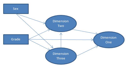
Figure 4.1: Structural Path Model Diagram
4.7.59 title
Specifies the title that is to appear at the top of any printed ACER ConQuest output.
4.7.60 while
Allows conditional execution of commands
4.7.60.1 Argument
(logical condition) {
set of ACER ConQuest commands
};
While logical condition evaluates to true the set of ACER ConQuest commands is executed. The commands are not executed if the logical condition does not evaluate to true.
The logical condition can be true, false or of the form s1 operator s2, where s1 and s2 are strings and operator is one of the following:
| Operator | Meaning |
|---|---|
| == | equality |
| => | greater than or equal to |
| >= | greater than or equal to |
| =< | less than or equal to |
| <= | less than or equal to |
| != | not equal to |
| > | greater than |
| < | less than |
For each of s1 and s2 ACER ConQuest first attempts to convert it to a numeric value. The numeric value can be a scalar value, a reference to an existing 1x1 matrix variable or a 1x1 submatrix of an existing matrix variable. A numeric value cannot involve computation.
If s1 is a numeric value the operator is applied numerically. If not a string comparison occurs between s1 and s2.
4.7.60.4 Example
x=fillmatrix(20,20,0);
compute k=1;
compute i=1;
while (i<=20)
{
for (j in 1:i)
 {
  if (j<i)
   {
    compute x[i,j]=k;
    compute x[j,i]=-k;
    compute k=k+1;
   };

  if (j==i)
   {
    compute x[i,j]=j;
   };
 };
compute i=i+1;
};
print x;
Creates a 20 by 20 matrix of zero values and then fills the lower triangle of the matrix with the numbers 1 to 190, the upper triangle with -1 to -190 and the diagonal with the numbers 1 to 20. The matrix is then printed to the screen.
4.8 Compute Command Operators and Functions
4.8.1 Operators
The standard binary mathematical operators are: addition (+),
subtraction (-), multiplication (*), and division (/).
All are available and operate according to their standard matrix definition
when applied to conformable matrices.
Division by a matrix is treated as multiplication by the matrix inverse.
If the operators are applied to non-conformable matrices then the operators
return a null matrix excepting when one of the arguments is a double
(or 1 by 1 matrix), then the operator is applied element-wise.
The unary negation operator (-) is available and is applied element wise to a matrix.
The exponentiation operator (^) is available but cannot be applied to matrices.
Two special binary mathematical operators are provided for element-wise matrix
multiplication (**) and division (//).
The ** operator multiplies each of the matching elements of two identically
dimensioned matrices. The // operator divides each element of the first
matrix by the matching element of the second matrix.
The following 6 logical operators are available:
| Operator | Meaning |
|---|---|
| == | equality |
| => | greater than or equal to |
| >= | greater than or equal to |
| =< | less than or equal to |
| <= | less than or equal to |
| != | not equal to |
| > | greater than |
| < | less than |
These operators are applied element-wise to a pair of matrices and return matrices of ‘1’ and ‘0’ with 1 if an element-wise comparison is true and 0 if it is false.
4.8.2 Standard Computation Functions for Matrices
The following standard functions are available. Each of the functions takes a single matrix argument and is applied element-wise to the matrix. Each function, therefore, returns a matrix of the same dimensions as the input.
abs(matrix)
Each element of the input matrix is a double.
Returns a matrix of the same dimensions as the input, matrix where
each element is the absolute value of the corresponding elements in the
input matrix.
ceil(matrix)
Each element of the input matrix is a double.
Returns a matrix of the same dimensions as the input, matrix where
each element is the ceiling of the corresponding elements in the
input matrix.
exp(matrix)
Each element of the input matrix is a double between 0 and 1.
Returns a matrix of the same dimensions as the input, matrix where
each element is exponent base e of the the corresponding element in the input
matrix.
floor(matrix)
Each element of the input, matrix is a double.
Returns a matrix of the same dimensions as the input, matrix where
each element is the floor of the corresponding elements in the
input matrix.
int(matrix)
Each element of the input matrix is a double.
Returns a matrix of the same dimensions as the input, matrix where
each element is the integer component of the corresponding elements in the
input matrix.
invgcdf(p)
Each element of the input matrix is a probability (a double between 0 and 1).
Returns a matrix of the same dimensions as the input, matrix where
each element is the inverse Gaussian distribution function for p.
log(matrix)
Each element of the input matrix is a double greater than 0.
Returns a matrix of the same dimensions as the input, matrix where
each element is the natural log of the corresponding element in the input
matrix.
log10(matrix)
Returns a matrix of the same dimensions as the input, matrix where
each element is the log base 10 of the corresponding element in the input
matrix. Each element of matrix must be greater than 0.
logit(matrix)
Returns a matrix of the same dimensions as the input, matrix where
each element is the logit of the corresponding element in the input
matrix. Each element of matrix must be between 0 and 1.
rnd(matrix)
Returns a matrix of the same dimensions as the input, matrix where
each element is the integer-rounded value of the corresponding elements in the
input matrix.
sqrt(matrix)
Returns a matrix of the same dimensions as the input, matrix where
each element is the square root of the corresponding element in the input
matrix. Each element of matrix must be greater than or equal to 0.
4.8.3 Accessing Matrix Information
Sub matrices can be extracted from matrices by
appending [rowstart:rowend,colstart:colend] to the name
of a matrix variable, for example m[2:5,5:10].
If all rows are required, rowstart and rowend can be omitted.
If all columns are required, colstart and colend can be omitted.
If a single row is required, rowend and the colon “:” can be omitted.
If a single column is required, colend and the colon “:” can be omitted.
Column and row indexing commence at one. So that,
for example, m[10,3] refers to the element in the 10-th row and 3-th column.
Single elements of a matrix can be specified to the left of the equal
operator ‘=’ by appending [row,col] to the name of a matrix variable.
Sub matrices cannot be specified to the left of the equal operator ‘=’.
4.8.4 Matrix Manipulation Functions
Two binary operators are available for concatenating matrices.
Column concatenation of two matrices, m1 and m2 is performed
using m1|^m2. In this case, m1 and m2 must have column
conformability and the matrix m1 is added under matrix m2.
Row concatenation of two matrices, m1 and m2 is performed
using m1->m2. In this case m1 and m2 must have row
conformability and the matrix m1 is added to the left of matrix m2.
Function arguments can themselves be functions or computed values but those functions or computed value must be enclosed in parentheses.
The following functions are available for manipulating the content of matrices:
counter(int)
Returns a matrix with dimensions int x 1 filled with integers running from 1 to int.
diag(matrix)
Returns the diagonal elements of the input, matrix: a square matrix.
fillmatrix(nrow,ncol,val)
Returns a matrix with dimensions nrow x ncol filled with the value val.
identity(arg)
Returns a matrix of dimension arg.
iif(arg1,arg2,arg3)
All three arguments must be matrices of the same dimensions.
The result is a matrix where an element takes its value from arg2 if the
matching arg1 element is ‘1’, otherwise it takes its value from arg3.
selectifcolumn(matrix,colref,val)
matrix is a matrix, colref is a column reference and, val is a value.
The result is a matrix that contains only those rows of matrix where column colref
takes value val.
transpose(matrix)
Transpose matrix of matrix.
vec(arg)
Returns a vector, which is the vec of arg.
vech(arg)
Returns a vector, which is the vech of arg.
inv(arg)
Inverse of matrix arg.
det(arg)
Determinant of matrix arg.
trace(arg)
Trace of matrix arg.
rows(arg)
Number of rows of matrix arg.
cols(arg)
Number of columns of matrix arg.
min(arg)
Number minimum of all elements in matrix arg.
max(arg)
Number maximum of all elements in matrix arg.
sum(arg)
Sum of all elements in matrix arg.
sum2(arg)
Sum of squares of all elements in matrix arg.
colcp(arg)
Column cross-products, returns a row × row matrix equal to arg*transpose(arg).
rowcp(arg)
Row cross-products, returns a column × column matrix equal to transpose(arg)*arg.
rowcov(arg)
Row covariance, returns a column × column matrix which is the covariance matrix of the columns.
rowcor(arg)
Row correlations, returns a column × column matrix which is the correlation matrix of the columns.
colsum(arg)
Returns a row which contains the sum over each of the columns of the arg.
rowsum(arg)
Returns a vector which contains the sum over each of the rows of the arg.
sort(arg)
Returns a vector which is contains the rows of arg sorted in ascending order.
The argument must be a vector.
long(matrix)
Takes in a matrix and returns a new matrix with dimensions:
- number of rows equal to (rows \(\times\) cols of
matrix) - 3 columns
Each row in the returned matrix represents an element of the original matrix. Column 1 of the returned matrix is the row number of the element of the original matrix. Column 2 of the returned matrix is the column number of the element of the original matrix. Column 3 of the returned matrix is the element (value) of the original matrix.
mod(m1,m2)
Takes 2 matrices as input and returns the element wise modulus.
percentiles(data,centiles)
Takes a matrix of data and returns a matrix of size rows of centiles x columns of
data.
The columns of the returned matrix are the percentiles of the columns of data.
4.8.5 Random Number Generators
The following random number generators are used. To control the seed use set seed =n.
rbernoulli(probs)
Matrix of Bernoulli variables where probs is a matrix of p values.
rchisq(df)
Chi square deviate with df degrees of freedom.
rint(min,max)
The integer component of a random uniform deviate from the range min and max.
Both min and max must be integers.
rinvshisq(df)
Inverse chi-square deviate with df degrees of freedom.
rlefttnormal(q)
Deviate from a standard normal left truncated at q.
rmvnormal(mu,var)
A random multivariate normal deviate with mean vector mu and covariance matrix covar.
rmvnmatrix(mu,sigma,nrow)
Returns a matrix of dimensions nrow by length of mu. Rows are
independent multivariate normal deviates with mean vector mu and covariance matrix sigma.
rnormal(mu,sd)
A random normal deviate with mean mu and standard deviation sd.
rnormalmatrix(mu,sd,nrow,ncol)
An nrow x ncol matrix of random deviates, with mean mu and standard deviation sd.
rpg(b,c)
A random deviate from a Pólya-gamma distribution with parameters “b” (int > 0)
and “c” (double).
rpgmatrix(b,c,nrow,ncol)
An nrow x ncol matrix of random deviates random deviates from a Pólya-gamma
distribution with parameters “b” (int > 0) and “c” (double).
rrighttnormal(q)
Deviate from a standard normal right truncated at q.
runiform(min,max)
A random uniform deviate from the range min and max.
runiformmatrix(min,max,nrow,ncol)
An nrow x ncol matrix of random unifomr deviates
from the range min and max.
4.9 Matrix Objects Created by Analysis Commands
A number of analysis returns can save their results in a family of matrix objects that are added to the ACER ConQuest variable list (see the command print). These variables then become available for manipulation or other use. Note that the matrix objects created cannot be directly modified by the user. The matrix objects can be, however, copied and then manipulated.
The commands that can produce matrix variables are: descriptives, estimate, fit generate, and matrixsampler.
For each of these commands the option matrixout=stem is used to request the variables and to set a prefix for their name.
The variables produced by each command and their format is provided below.
All matrix objects created have a user-specified prefix, followed by an underscore (“_“), followed by a suffix as defined for each command below.
4.9.1 Descriptives Command
The following four matrices are produced regardless of the estimator option:
- descriptives
Number of dimensions by eight, providing for each dimension the dimension number, number of cases, mean, standard deviation, variance, standard error of the mean, standard error of the standard deviation, and standard error of the variance. - percentiles
Number of dimensions by the number of requested percentiles plus two, providing for each dimension the dimension number, number of cases, and then each of the percentiles. - bands
Number of dimensions by twice the number of requested bands plus two, providing for each dimension the dimension number, number of cases, and then proportion in each of the bands follow by standard errors for each of the band proportions. - bench
Number of dimensions by four, providing for each dimension the dimension number, number of cases, proportion below the benchmark and standard error of that proportion.
If latent is chosen as the estimator then in addition to the above the following matrices are available:
- pv_descriptives
Number of dimensions times number of plausible values by six, providing for each dimension and plausible value, the dimension number, the plausible value number, number of cases, mean, standard deviation, and variance. - pv_percentiles
Number of dimensions times number of plausible values by the number of percentiles plus three, providing for each dimension and plausible value, the dimension number, the plausible value number, number of cases, and then each of the percentiles. - pv_bands
Number of dimensions times number of plausible values by the number of requested bands plus three, providing for each dimension and plausible value, the dimension number, the plausible value number, number of cases, and then proportion in each of the bands.
4.9.2 Estimate Command
Regardless of the options to the command estimate used, the following two matrices are produced:
- xsi
A single column of the estimated item location parameters. - history
Number of iterations by total number of estimated parameters plus three. The first column is the run number. The second column is the iteration number within the run. The third column is the deviance. The remaining columns are for the parameter estimates.
If the model includes estimated scoring parameters, then the following matrix is also produced:
- tau
A single column of the estimated item scoring parameters.
Depending on the options specified the following matrices are also available:
If the method=jml option is chosen or abilities=yes in conjunction with an MML
method then the following two matrices of case estimates are produced.
- mle
Number of cases by number of dimensions providing for each case the MLE latent estimate for each case. - wle
Number of cases by number of dimensions providing for each case the WLE latent estimate for each case.
If abilities=yes is used in conjunction with an MML method, or MCMC estimation
is used, then a matrix of case plausible values and a matrix of case EAPs is produced.
pvs
Number of cases by number of dimensions times number of plausible values. For the columns the plausible values cycle fastest. For example, if there are three dimensions and two plausible values, column one would contain plausible value one for dimension one, column two would contain plausible value two for dimension one, column three would contain plausible value one for dimension two and so on.eap
Number of cases by number of dimensions.
If ifit=yes is used (the default) a matrix of item fit values is produced.
- itemfit
Number of fit test by four. The four columns are the unweighted T, weighted T, unweighted MNSQ, and weighted MNSQ.
If pfit=yes is used a matrix of case fit values is produced.
- casefit
Number of cases by one. Providing for each case the unweighted mean square.
If stderr=empirical is used (the default for MML) then the estimate error covariance matrix is produced.
- estimatecovariances
A number of parameter by number of parameter matrix of estimate error covariances.
If stderr=quick is used (the default for JML) then the following estimate error variances
matrix objects are produced.
- xsierrors
Number of item location parameter estimates by one, providing for each item location parameter the associated estimate variance. - regressionerrors
Number of regression parameters by one, providing for each regression parameter the estimate variance. - covarianceerrors
Number of covariance parameters by one, providing for each regression parameter the estimate variance.
And, if item scoring parameters are estimated,
- tauerrors
Number of item scoring parameters by one, providing for each item scoring parameter the associated estimate variance.
4.9.3 Fit Command
Produces a set of matrices, one for each level of the group used in the group=option.
- userfit
Each matrix with the suffix userfit will be preceded by the group name as well as the user defined prefix. Each matrix (one per group) has dimension number of fit tests by four, providing for each test the un-weighted t-fit, weighted t-fit, un-weighted mean square and weighted mean square.
4.9.4 Generate Command
The matrices that are produced by generate depend upon the options chosen. Regardless of the options chosen the following matrix is produced:
- items
Number of items by three, providing for each item the item number, category number, and the generated parameter value.
If the option scoresdist is used then a matrix of scoring parameters is produced.
- scores
Number of total item scoring categories by number of dimensions plus two, providing for each item category, the item number, category number and score for each dimension.
If the option importnpvs is NOT used then the following two matrices are produced:
- responses
Number of cases by number of items, providing for each case a response to each item. - cases
Number of cases by number of dimensions plus one, providing for each case a case number and a generated ability for each of the dimensions.
If the option importnpvs is used then the following matrices of summary statistics are produced for each dimension and group:
- statistics
Number of plausible values by three times the number of items plus three. It contains mean raw scores, raw score variances, Cronbach’s alpha and then for each item, mean item score and point biserial statistics (biased and unbiased).
4.9.5 Itanal Command
Produces a set of matrices, one for each level of the group used in the group=option.
The name of the matrix is provided by the matrixout=option. The matrices produced are as follows.
- counts Number of items by number of response categories, providing for each item, the frequency of responses in each category.
- itemstats Number of items by six, providing for each item: item-total correlations, item-rest correlations, observed mean score, expected mean score, adjusted mean score, and item delta dot. For details see command itanal.
- ptbis
Number of items by three times the number of response categories,
providing for each item and category the:
- point-biserial correlation with the total score,
- the t-test of the point-biserial, and
- the associated p value.
- abilitymeansd Number of items by number of response categories by dimension by two, providing for each item, category, and dimension the mean and standard deviation of the ability estimate (when using PVs the first plausible value is used) of the cases who responded in that category.
- summarystats Descriptive statistics for the raw scores. Matrix is one by ten. Percent Missing, N, Mean, SD, Variance, Skew, Kurtosis, Standard error of mean, Standard error of measurement, Alpha.
4.9.6 Matrixsampler Command
Produces matrices with the name provided in the matrixout=option.
This produces all of the matrices produced under the itanal command, plus one that
contains descriptive statistics for simulated data, one that contains fit statistics
for the user’s data, and one that contains fit statistics for simulated data. The two matricies (fit and userfit) containing fit statistics are only provided if fit=yes is specified in the command.
- raw
contains a row for each sampled matrix and columns providing the inter-item and item-total correlations. - inputfit
contains a row for each parameter and sampled matrix combination and columns Unweighted_t, Weighted_t, Unweighted_MNSQ, Weighted_MNSQ, Parameter and replication Set. - samplerfit
contains a row for each parameter and columns: Unweighted_t, Weighted_t, Unweighted_MNSQ, Weighted_MNSQ, Parameter number. These are the estimates from the analysis of the user’s dataset.
4.9.7 Structural Command
Produces a set of matrices, one for each regression model and four matrices of sums of squares and cross-products. The name of the matrix is provided by the matrixout=option. The matrices produced are as follows.
- fullsscp
Square matrix with dimension equal to the total number of variables in the structural model providing the sums of squares and cross-products. - osscp
Square matrix with dimension equal to the number of observed variables (non latent variables) in the structural model providing the sums of squares and cross-products. - losscp
Number of latent by number of observed variables providing the cross-products. - lsscp
Square matrix with dimension equal to the total number of latent variables in the structural model providing the sums of squares and cross-products. - results_eqnn
Where the matrix object contains the results of the estimation of each of the n regression equations in the structural model. The cell 1,1 contains the R-squared, and there are additional rows for each independent variable, column one of each of those additional rows is the estimated regression parameter and the second column is its standard error estimate.
4.10 List of Illegal Characters and Words for Variable Names
| Character |
|---|
| | |
| / |
| $ |
| ~ |
| Term | Type |
|---|---|
| all | Word |
| category | Word |
| dimensions | Word |
| fitstatistics | Word |
| on | Word |
| parameters | Word |
| step | Word |
| steps | Word |
| to | Word |
| tokens | Word |
| variables | Word |
| abs | Function |
| ceil | Function |
| colcp | Function |
| cols | Function |
| colsum | Function |
| counter | Function |
| det | Function |
| exp | Function |
| fillmatrix | Function |
| floor | Function |
| identity | Function |
| iif | Function |
| int | Function |
| inv | Function |
| log | Function |
| log10 | Function |
| logit | Function |
| max | Function |
| min | Function |
| percentiles | Function |
| rbernoulli | Function |
| rchisq | Function |
| rinvchisq | Function |
| rleftnormal | Function |
| rmvnormal | Function |
| rnd | Function |
| rnormal | Function |
| rnormalmatrix | Function |
| rowcor | Function |
| rowcov | Function |
| rowcp | Function |
| rows | Function |
| rowsum | Function |
| rpg | Function |
| rpgmatrix | Function |
| rrightnormal | Function |
| runiform | Function |
| runiform | Function |
| selectifcolumn | Function |
| sort | Function |
| sqrt | Function |
| sum | Function |
| sum2 | Function |
| trace | Function |
| transpose | Function |
| banddefine | Command name |
| build | Command name |
| caseweight | Command name |
| categorise | Command name |
| chistory | Command name |
| clear | Command name |
| codes | Command name |
| compute | Command name |
| datafile | Command name |
| delete | Command name |
| descriptives | Command name |
| directory | Command name |
| display | Command name |
| dofor | Command name |
| doif | Command name |
| dropcases | Command name |
| else | Command name |
| enddo | Command name |
| endif | Command name |
| equivalence | Command name |
| estimates | Command name |
| execute | Command name |
| exit | Command name |
| export | Command name |
| facets | Command name |
| filter | Command name |
| fit | Command name |
| for | Command name |
| format | Command name |
| function | Command name |
| generate | Command name |
| get | Command name |
| gingroup | Command name |
| group | Command name |
| if | Command name |
| import | Command name |
| itanal | Command name |
| keepcases | Command name |
| key | Command name |
| kidmap | Command name |
| labels | Command name |
| let | Command name |
| matrixsampler | Command name |
| mh | Command name |
| missing | Command name |
| model | Command name |
| plot | Command name |
| Command name | |
| put | Command name |
| quit | Command name |
| read | Command name |
| recodes | Command name |
| regression | Command name |
| reset | Command name |
| scatter | Command name |
| scores | Command name |
| set | Command name |
| show | Command name |
| structural | Command name |
| submit | Command name |
| system | Command name |
| systemclean | Command name |
| timerstart | Command name |
| timerstop | Command name |
| title | Command name |
| while | Command name |
| write | Command name |
The suffixes added to matrix objects created using the option “matrixout” are also protected words. These suffices cannot be within declarations (e.g., a sub string of the declaration).
| Term | Type |
|---|---|
| _bands | Extension |
| _bench | Extension |
| _casefit | Extension |
| _cases | Extension |
| _counts | Extension |
| _covarianceerrors | Extension |
| _descriptives | Extension |
| _estimatecovariances | Extension |
| _fullsscp | Extension |
| _history | Extension |
| _inputfit | Extension |
| _itemerrors | Extension |
| _itemfit | Extension |
| _itemparams | Extension |
| _items | Extension |
| _itemtotrestcor | Extension |
| _losscp | Extension |
| _lsscp | Extension |
| _mle | Extension |
| _osscp | Extension |
| _percentiles | Extension |
| _ptbis | Extension |
| _pv_bands | Extension |
| _pv_descriptives | Extension |
| _pv_percentiles | Extension |
| _pvmeansd | Extension |
| _pvs | Extension |
| _raw | Extension |
| _regressionerrors | Extension |
| _responses | Extension |
| _results_eqn | Extension |
| _samplerfit | Extension |
| _scores | Extension |
| _statistics | Extension |
| _userfit | Extension |
| _wle | Extension |
![]()
Note that both of these examples assume you have navigated to the path of your ACER ConQuest install and that your command file is in the same location.↩︎